This Mathematica notebook explains the derivation of the Landau-Lifshitz pseudotensor, a mathematical object used to describe the energy and momentum of a gravitational field in general relativity. Although not a true tensor, as it depends on the choice of coordinates and cannot be localized, the pseudotensor has useful properties such as being symmetric, having zero divergence in flat spacetime, and being conserved in asymptotically flat spacetime. The concept of the stress-energy-momentum (SEM) tensor is introduced, which is a true tensor that combines energy, mass, momentum, and their fluxes and stresses. Derived from the action principle, the SEM tensor satisfies conservation law in flat spacetime. However, in curved spacetime, it is not conserved due to the presence of a gravitational field. A pseudotensor that locally has zero divergence is then found and corrected for curvature effects. The pseudotensor can be obtained in terms of second derivatives of the metric tensor, which characterizes the geometry of spacetime. It is constructed from the Einstein tensor, related to the Ricci tensor and Ricci scalar, which are in turn related to the Riemann tensor containing all information about spacetime curvature. A computer algebra system called xTensor is used to perform calculations and simplify expressions. Another way to obtain the pseudotensor is in terms of first derivatives of the metric tensor. This form is more convenient for some applications such as calculating gravitational radiation emitted by a system. The pseudotensor can also be obtained in terms of first derivatives of the metric density, a modified version of the metric tensor that includes a factor of $\sqrt{-g}$ where $g$ is the determinant of the metric tensor. Preferred by some authors because it makes integration over curved spacetime easier, this factor is related to the Jacobian determinant of coordinate transformations and affects the volume element. Another way to obtain the pseudotensor is in terms of Christoffel symbols, which describe spacetime curvature. Related to first derivatives of the metric tensor, they are used to define covariant derivatives invariant under coordinate transformations. xTensor is used to perform calculations and compare them with EinS. The notebook concludes with remarks on the physical meaning and interpretation of the pseudotensor and mentions alternative definitions and approaches for finding a pseudotensor that can describe energy and momentum of a gravitational field in general relativity.
The Landau-Lifshitz pseudotensor,
A complex concept to remember.
The stress-energy distribution
Is to the gravity contribution.
It's a mathematical tool,
To study the gravitational pool,
It helps us understand,
The space-time curvature at hand.
It's a subtle concept, not easy to grasp,
But it holds the key, to unlock the past,
Of our understanding, of the universe,
And the forces that govern it, diverse.
So let us honor Landau-Lifshitz,
By delving in their study which is
About gravity, and the laws involved,
And get this pseudotensor solved.
Anonymous
This Mathematica notebook is a detailed workout of the main part of [1] (the Book). The derivation of Landau-Lifshitz pseudotensor is rightly considered as one of the hardest and most calculation-intensive parts of the Book. This is especially true for the calculation of the pseudotensor in terms of Christoffels (eq. LL96,8) and metric densities (eq. LL96,9)(LL
in front of the equation number means that the equation is from the Book). The Book chapter §96 starts with relatively simple expressions but very quickly they turn into a morass of indices through substitutions and decompositions. The calculation of the final formulae can proceed by several different paths with branching in different steps of the calculation chain. A somewhat different and quite original approach for finding a similar pseudotensor is pursued the J.L.Synge' s masterpiece [2], where a surprising shortcut avoids a large part of the tedium. In a subsequent post, I'll show evidence that Synge's pseudotensor is somewhat different than the Landau-Lifshitz (LL) pseudotensor despite the widespread opinion that they are just different derivations of the same pseudotensor.
Computations in this research field, although relatively uncomplicated, were not, until recently, amenable to computer algebra treatment because most tensor packages in general purpose programs, such as Mathematica and Maple, hadn't the full capability to work directly with indexed tensors (indicial notation) and most functions acted on components. This involved conversion of indexed tensors to matrices of components and operation with the matrices, which is computationally intensive and in many cases, not really required. On the other hand, tensor algebra in textbooks and papers is performed on indexed tensors, whose component structure in many cases is not known or not relevant for the problem at hand. More recent tensor packages, like Tensorial and xTensor for Mathematica, Riegeom for Maple, and itensor (indicial tensor) for Maxima allow direct manipulation of indexed tensors. The following exposition uses xTensor by José M.Martín - García at the xAct site and some of the accompanying packages. The software version used is Mathematica 11.0. The Landau-Lifshitz pseudotensor example is a good test of xTensor as it clearly outlines its strong and weak points.
The simplification procedures in the package xTensor are automated to a very large degree and use the so-called "canonicalization", a process in which individual terms in a tensor sum are converted in some canonical form that makes them more uniform and non-reducible. On the other hand, automatism means less transparency. Therefore, when deriving LL96,8 and LL96,9 the automatic routine will be accompanied with somewhat less automatic and more transparent calculations.
Energy and momentum conservation principle in general relativity
Two of the most popular definitions of the combined Energy and Momentum Conservation Principle (EMCP) are:
- the energy and momentum of a closed isolated system are conserved
- the stress - energy - momentum tensor of a closed isolated system is a constant quantity
The second definition is preferred in theoretical physics. The stress-energy-momentum (SEM) tensor, $T^k_i$, that combines energy, mass, momentum, their fluxes and stresses (also called "super energy-momentum tensor", etc.), is the content of the Universe. It is both the matter and the electromagnetic fields. SEM is derived by varying the action integral and is defined in eq. LL32,3 as:
$$T_i^k = q_{,i}\frac{\partial \Lambda }{\partial q_{,k}} - \Lambda \delta _i^k$$where Λ is the Lagrange function and q is a generalised coordinate. EMCP requires that the SEM tensor is constant. Imagine the closed isolated system as a volume (Universe, black hole), enclosed by an impenetrable envelope such that no matter or radiation can pass through. The SEM tensor within the enclosed volume is constant: there is no tensor flow through the envelope. Tensor flow, or tensor divergence, is the sum of partial derivatives of tensor components with respect to coordinates (similar to vector divergence). From the equations of motion it follows that divergence should be zero according to LL32,4:
$$\frac{\partial T_i^k}{\partial x^k} = T_{i,k}^k = 0$$which is, of course, the EMCP. In the middle of the above equation the ordinary derivatives are given with the simpler comma notation. In a similar mood, covariant derivatives will be marked with semi-colons.
Presence of gravitation spoils this clear picture in several ways. Gravitation curves space. In curved space, tensor (and vector) flows are ill-defined because they change direction in each point. Parallel transfer, which is essential for definition of derivatives, is very complicated on curved paths. Derivatives are only obtained after making corrections for the curvature – one correction for each tensor index. These corrected derivatives are known as covariant derivatives. In curved space, ordinary derivatives are replaced by covariant ones:
$$ T_i^l \Gamma _{kl}^k -\Gamma _{ik}^l T_l^k+\frac{\partial T_i^k}{\partial x^k} \equiv T_{i;k}^k $$But $T^{ik}$ is a symmetric tensor, and, according to eq. LL86,11 the above becomes (eq. LL96,1):
$$T_{i;k}^k=\frac{1}{\sqrt{-g}} \frac{\partial \sqrt{-g} T_i^k}{\partial x^k} - \frac{1}{2}T^{kl}\frac{\partial g_{kl}}{\partial x^i}$$Does this equation express the conservation of energy and momentum in curved space-time or, in other words, can it be turned to zero? The answer is emphatically NO and that' s why : Let $T^{ik}$ be the true stress - energy tensor and $P^i$ be the 4-momentum (energy + momentum) of the system that must be a conserved quantity. By an analogy with eq. LL32,6
$$P^i=\frac{1}{c} \int \sqrt{-g} T^{ik} dS_k$$where $\sqrt{-g}dS_k$ is the element of a hypersphere in a curved plane. In order to make the expression for $P^k$ exactly identical to that in eq. LL32, 6, $T^{ik}$ should be equated to the stress-energy of the system (this is only by analogy, and does not reflect the tensor properties of $T^{ik}$, as the Book footnote warns). Then, in order to conserve the 4-vector $P^i$, the integral (LL32,6) must be conserved over the whole hyperplane, that is, over the whole 3-dimensional space. As proved in Book, Ch. 29 with the help of Gauss theorem, the integrand must fulfill the following condition in order to conserve the integral:
$$\frac{\partial T^{ik}}{\partial x^k} = 0.$$This condition is not, however, met in eq. LL96,1, where the additional term $-\frac{1}{2} T^{kl} \frac{\partial g_{kl}}{\partial x^i}$ and the presence of $\sqrt{-g}$ around $T^{ik}$ do not allow derivation of a global conservation law in a manner, analogous to the Classical Field Theory. This is so, because the gravitational field is also a component of $T^{ik}$ which should be included inside it, together with pure matter and electromagnetic field. The offending terms cannot be eliminated because the metric tensor $g^{ik}$ is not constant – it can be anything, depending on the spacetime topology. So, in the first term in the right hand side $\sqrt{-g}$ cannot be pulled out from inside the differential operator. However, the real difficulty lies in the term $-\frac{1}{2} T^{kl} \frac{\partial g_{kl}}{\partial x^i}.$
Taking up the above analogy, the volume that contains the SEM tensor itself stretches, shrinks, and moves in every imaginable way. It cannot be bound in an envelope with zero volume. The spacetime itself generates tensor flows. Do what you want, you can’t just ignore or remove the second term. Failure to do so means nothing less than the startling conclusion: in the curved spacetime of general relativity, the EMCP is no longer valid. Whether this is real or apparent remains subject to interpretation. It is easy to see, however, that this result can be expected from what we know from elementary physics. In the heart of the concept of the energy conservation principle is the assumption that space is isotropic while the momentum conservation principle requires symmetric space. Both isotropy and symmetry are no longer assumed in curved spacetime. The energy and momentum conservation principles fail in principle. The very basis on which they are built sinks into a quicksand. Is there a way to salvage something?
In search of symmetry
Many efforts have been and are being made to sidetrack this important unsolvable problem. Landau-Lifshitz turned their attention to a couple of possible loopholes.
First, as pointed by Einstein, it is always possible to flatten the space (make it pseudo-Euclidean) in the neighbourhood of a point (locally), or, in other words, it is always possible to locally extinguish the field by, e.g., choosing such a frame that all first derivatives of the metric $\frac{\partial g_{ik}}{\partial x^l} \equiv g_{ik,l}$ vanish. Then, at this point, the second term in (LL96,1) disappears and by dint of eq. 86,4 : $\frac{\partial g}{\partial x^l} = gg^{ik} g_{ik,l}$, the first derivatives of g also vanish. Equation LL96,1:$$T{}_{i;k}^k=\frac{1}{\sqrt{-g}}\frac{\partial \left(\sqrt{-g} T_i^k\right)}{\partial x^k}-\frac{1}{2}T^{kl} \frac{\partial g_{kl}}{\partial x^i}$$
becomes after eliminating the first derivatives of the metric and metric determinant:
$$T{}_{i;k}^k=\frac{\partial T_i^k}{\partial x^k}=T{}_{i,k}^k$$so that the offending terms disappear; this means that the tiny volume around this point can be enclosed in an envelope into which EMCP is valid. In contravariant form it is:
$$\frac{\partial T^{ik}}{\partial x^k} = 0$$Second, the above identity does not fix $T^{ik}$ exactly but leaves a quantity undefined. Namely, according to LL32,7, one can always find an antisymmetric tensor $\eta^{ikl} = -\eta^{ilk}$ such that if $T^{ik} = \eta^{ikl}{}_{,l}$ then $T^{ik}{}_{,k} = \eta^{ikl}{}_{,lk} \equiv 0$. It makes use of the fact that the second derivatives of any antisymmetric tensor disappear because of the symmetry of the differentiation operator. We prove this with the automatic simplification routine of xTensor:
DefTensor[η[i,k,l],M4,Antisymmetric[{2,3}]];
** DefTensor: Defining tensor η[i,k,l].
differentiate the above twice by k and l, equate to 0, canonicalize and check if true:(PD[-l]@PD[-k]@η[i,k,l] == 0) // ToCanonical
true
which proves the identity.The possibility to locally fulfill EMCP gives the idea to find a SEM tensor that locally has a zero divergence and then correct it to make it valid globally, in curved spacetime. An inkling to the nature of this correction may be taken from the analogous case with the covariant derivatives. There all corrections contain Christoffel symbols which are composed from first derivatives of the metric tensor. The way to make the required SEM tensor is already obvious: it must be such antisymmetric expression that upon differentiation becomes a second derivative which is identically zero. When constructing it, we must throw out all first metric derivatives that would prevent the expression from turning to zero. To put $T^{ik}$ into the required form ($T^{ik} = \eta^{ikl}{}_{,l}$), Landau & Lifshitz use the right-hand side of the field (Einstein) equations (LL95,5) in contravariant form
RHSEinstein = EinsteinCD[i, k] // EinsteinToRicci
$$R^{ik}-\frac{1}{2}g^{ik}R$$
Define Ricci tensor and Ricci scalar in terms of Riemann tensor
RicciToRiemann = RicciCD[i_, k_] :> metricg[i, m] metricg[k, p] metricg[l, n] RiemannCD[-l, -m, -n, -p];
RicciScalarToRiemann = RicciScalarCD[] :> metricg[l, n] metricg[m, p] RiemannCD[-l, -m, -n, -p];
Decompose the Einstein tensor as usual to Ricci tensor and Ricci scalar and then turn them to Riemann tensor using the above definitions. The Ricci tensor is substituted according to (LL92,9) and the scalar curvature according to (LL92,12) both in terms of the Riemann tensor.
RHSEinstein /. RicciToRiemann;
Energy = % //. RicciScalarToRiemann // Expand
$$g^{im} g^{kp} g^{ln} R_{lmnp} - \tfrac{1}{2} g^{ik} g^{ln} g^{mp} R_{lmnp}$$
Define Riemann tensor as second metric derivatives and Christoffel symbols (first metric derivatives) according to LL92, 1.
RiemannSecondDerivatives = RiemannCD[-i_, -k_, -l_, -m_] :> 1/2 (-PD[-m][PD[-k][metricg[-i, -l]]] + PD[-l][PD[-k][metricg[-i, -m]]] + PD[-m][PD[-i][metricg[-k, -l]]] - PD[-l][PD[-i][metricg[-k, -m]]]) + metricg[-r, -q] (ChristoffelCD[r, -k, -l] ChristoffelCD[ q, -i, -m] - ChristoffelCD[r, -k, -m] ChristoffelCD[q, -i, -l]);
Express the curvature part of the Einstein equations (the Einstein tensor) as second metric derivatives and Christoffels
EnergyTensor = Energy /. RiemannSecondDerivatives // ToCanonical
$$ \begin{align} \Gamma^{l}{}_{mn} \Gamma^{p}{}_{qr} g^{im} g^{kq} g_{lp} g^{nr} - \tfrac{1}{2} \Gamma^{l}{}_{mn} \Gamma^{p}{}_{qr} g^{ik} g_{lp} g^{mq} g^{nr} - \Gamma^{l}{}_{mn} \Gamma^{p}{}_{qr} g^{im} g^{kn} g_{lp} g^{qr} + \\ \tfrac{1}{2} \Gamma^{l}{}_{mn} \Gamma^{p}{}_{qr} g^{ik} g_{lp} g^{mn} g^{qr} - \tfrac{1}{2} g^{il} g^{km} g^{np} g_{np}{}_{,l}{}_{,m} + \tfrac{1}{2} g^{il} g^{km} g^{np} g_{mn}{}_{,l}{}_{,p} + \tfrac{1}{2} g^{il} g^{km} g^{np} g_{ln}{}_{,m}{}_{,p} - \\ \tfrac{1}{2} g^{ik} g^{lm} g^{np} g_{ln}{}_{,m}{}_{,p} - \tfrac{1}{2} g^{il} g^{km} g^{np} g_{lm}{}_{,n}{}_{,p} + \tfrac{1}{2} g^{ik} g^{lm} g^{np} g_{lm}{}_{,n}{}_{,p} \end{align} $$
In the locality first-order derivatives disappear (this means that the Christoffel-containing terms also disappear) which leaves only terms with second-order derivatives (step 1 elimination of first-order derivatives)
% /. {ChristoffelCD[l_, -m_, -n_] -> 0}
$$ -g^{il} g^{km} g^{np} g_{np,m,l} + g^{il} g^{km} g^{np} g_{mn,p,l} + g^{il} g^{km} g^{np} g_{ln,p,m} - g^{ik} g^{lm} g^{np} g_{ln,p,m} - g^{il} g^{km} g^{np} g_{lm,p,n} + g^{ik} g^{lm} g^{np} g_{lm,p,n} $$
Now the dummy indices are shuffled in such a way that the covariant tensors all become $g_{np,m,l}$ and the whole expression is factored
$$ \left ( -g^{il} g^{km} g^{np} + g^{il} g^{kp} g^{mn} + g^{ip} g^{kl} g^{mn} - g^{ik} g^{lp} g^{mn} - g^{in} g^{kp} g^{lm} + g^{ik} g^{np} g^{lm} \right ) g_{np,m,l} $$
The expression in parenthesis can be abbreviated as a 6-rank tensor $W^{iklmnp}$
$$W^{iklmnp} = -g^{il} g^{km} g^{np} + g^{il} g^{kp} g^{mn} + g^{ip} g^{kl} g^{mn} - g^{ik} g^{lp} g^{mn} - g^{in} g^{kp} g^{lm} + g^{ik} g^{np} g^{lm} $$and according to the well-known formula from calculus, the differentiation can be distributed over the product:
$$g_{np,m,l} W^{iklmnp} = \left ( g_{np,m} W^{iklmnp} \right ){}_{,l} - g_{np,m} W^{iklmnp}{}_{,l} $$The second term in the right-hand side disappears, because it contains first-order metric derivatives (step 2 elimination of first-order derivatives), and $W^{iklmnp}$ is substituted back. The expression in parentheses becomes:
$$ -g^{il} g^{km} g^{np} g_{np,m} + g^{il} g^{kp} g^{mn} g_{np,m} + g^{ip} g^{kl} g^{mn} g_{np,m} - g^{ik} g^{lp} g^{mn} g_{np,m} - g^{in} g^{kp} g^{lm} g_{np,m} + g^{ik} g^{np} g^{lm} g_{np,m} $$With the help of (LL86, 7): $g^{ln} g_{np,m} = -g_{np} g_{,m}^{ln}$ and (LL86, 4): $g_{,m} = gg^{np} g_{np,m}$, so that $g^{np} g_{np,m} = g_{,m} /g$
$$-\frac{g_{,m} g^{il} g^{km}}{g} + \frac{g_{,m} g^{ik} g^{ml}}{g} + g^{kp}g^{ml}g_{np}g_{,m}^{in} -g^{ip}g^{kl}g_{np}g_{,m}^{mn} - g^{il}g^{kp}g_{np}g_{,m}^{mn} + g^{ik}g^{lp}g_{np}g_{,m}^{mn}$$(LL83, 10): $g^{kp} g_{np} = \delta_n^k$, where $\delta_n^k$ is the Kronecker symbol
$-\frac{g_{,m}g^{il}g^{km}}{g} + \frac{g_{,m}g^{ik}g^{ml}}{g} + g^{ml}g_{,m}^{in}\delta_n^k -g^{kl}g_{,m}^{mn}\delta_n^i-g^{il}g_{,m}^{mn}\delta_n^k + g^{ik}g_{,m}^{mn}\delta_n^l$A property of the Kronecker symbol is $\delta _n^i g_{,m}^{mn} = g_{,m}^{im}$
$-\frac{g_{,m}g^{il}g^{km}}{g} + \frac{g_{,m}g^{ik}g^{ml}}{g} + g^{ml}g_{,m}^{ik} -g^{kl}g_{,m}^{im}-g^{il}g_{,m}^{km} + g^{ik}g_{,m}^{lm}$l and m are dummy indices in the whole expression (when it is doubly differentiated) which allows exchanging their places
$-\frac{g_{,m}g^{il}g^{km}}{g} + \frac{g_{,m}g^{ik}g^{lm}}{g} + g^{lm}g_{,m}^{ik} -g^{km}g_{,m}^{il}-g^{il}g_{,m}^{km} + g^{ik}g_{,m}^{lm}$The calculus formula for differentiation of a product (in reverse):
$-\frac{g_{,m} g^{il} g^{km} }{g} + \frac{g_{,m} g^{ik} g^{lm} }{g} + \left( g^{ik} g^{lm} \right)_{,m} - \left( g^{il} g^{km} \right)_{,m}$The distributive property of the differentiation operator, collection of $g_{,m}$, and substitution $U^{iklm} = g^{ik}g^{lm} - g^{il} g^{km}$
$\frac{1}{g} g_{,m} \left( g^{ik} g^{lm} - g^{il} g^{km} \right) + \left( g^{ik} g^{lm} -g^{il} g^{km} \right)_{,m} = \frac{1}{g} g_{,m} \left( U^{iklm} \right) + \left ( U^{iklm} \right )_{,m}$Once more the calculus formula for differentiation of a product in reverse and substitutions of $g_{,m} = -(-g)_{,m}$ and $g = -(-g)$
$\frac{1}{(-g)} \left [ (-g) U^{iklm} \right ]_{,m} = \frac{1}{(-g)} \left [(-g) \left( g^{ik} g^{lm} - g^{il} g^{km} \right )\right ]_{,m}$This leads to (LL96, 2) for $h^{ikl} = \frac{\partial}{\partial x^m} \lambda^{iklm}$, which is the numerator of the above expression, multiplied by the constant $\frac{c^4}{16 \pi k}$
It is easy to check (LL96, 4) $h^{ikl} = -h^{ilk}$. With a precision to a constant factor, $h^{ikl}$ corresponds to the expression in the parentheses of the term $(g_{np,m} W^{iklmnp}){}_{,l}$. The factor 1/(–g) is also a constant in the local case, so it can be pulled from under the operator ,l. For the whole term, which corresponds to the stress-energy tensor in the neighborhood of a point, thus
$\frac{1}{(-g)} h^{ikl}{}_{,l} = T^{ik}$
$ h^{ikl}{}_{,l} = (-g) T^{ik}$
$ (-g) T^{ik} = \frac{c^4}{16 \pi k} \left [ (-g) \left ( g^{ik} g^{lm} - g^{il} g^{km} \right ) \right ]_{,m,l}$
To summarize, the final expression for the SEM tensor in the special point as a result of the above transformations is:
$\frac{16 \pi k}{c^4} T^{ik} = \frac{1}{(-g)} \left [(-g) \left( g^{ik} g^{lm} - g^{il} g^{km} \right) \right]_{,m,l}$For the following discussion we need this expression somewhat rearranged. Namely, the constant $\frac{c^4}{16 \pi k}$ is put under ,l (but not under ,m) and both sides are multiplied by (−g). After these "simple transformations" (according to Landau-Lifshitz), we obtained a SEM tensor in a completely antisymmetric form:
$(-g) T^{ik} = \left\{ \frac{c^4}{16 \pi k} \left[(-g) \left(g^{ik} g^{lm} - g^{il} g^{km} \right) \right]_{,m} \right\}_{,l}$The quantity in the braces corresponds to $h^{ikl} = \eta^{ikl}$
$\eta^{ikl} = \frac{c^4}{16 \pi k} \left[(-g) \left(g^{ik} g^{lm} - g^{il} g^{km} \right) \right]_{,m}$and is antisymmetric for indices k, l while the quantity under the brackets corresponds to (LL96,3)
$\lambda^{iklm} = \frac{c^4}{16 \pi k} (-g) \left(g^{ik} g^{lm} -g^{il} g^{km} \right)$Note that first order derivatives we eliminated at two steps. $(−g)T^{ik}$ vanishes upon differentiation by ,k (obeys EMCP) as checked below. As seen from above
$(-g)T^{ik}{}_{,k} = \eta^{ikl}{}_{,l,k}$and $\eta^{ikl}{}_{,l,k} \equiv 0$ as proven above. To prove that $\eta^{ikl}$ also disappears in the metric form when doubly differentiated
etaikl = PD[-m][-Detmetricg[]*(metricg[i, k]*
metricg[l, m] - metricg[i, l]*metricg[k, m])];
Simplification[PD[-l]@PD[-k]@etaikl] == 0
true
Finally, let's prove that $T^{ik}$ expressed in metric derivatives is symmetric
gTik = PD[-l][
PD[-m][-Detmetricg[] (metricg[i, k] metricg[l, m] -
metricg[i, l] metricg[k, m])]];
ToCanonical[Antisymmetrize[gTik]] == 0
true
Landau-Lifshitz pseudotensor in canonical form
The nice and pliable SEM tensor obtained above whose divergence disappears automatically just by dint of symmetry (or, more precisely, antisymmetry) so that it fulfills EMCP, does not work outside the very small flat locality of the point that we chose. Remember that in its derivation above we threw out first derivatives of the metric tensor at a few steps. First derivatives usually combine to form connections (Christoffel symbols) and these last are directly connected to curvature. So we may expect that outside our flat neighborhood first derivatives will reappear to play a prominent role as corrections for curvature in the same way as they act in covariant derivatives. We have every reason to expect, then, that $(-g) T^{ik}$ will no longer be equal to $\eta_{,l}^{ikl}$ but there will be some non-zero difference that is the quantity that corrects for the transition from local to global geometry, from flat to curved spacetime: $\eta_{,l}^{ikl} - (-g) T^{ik} \neq 0$. Let’s define this difference as $(−g) t^{ik}$; then by definition $(-g) \left( T^{ik} + t^{ik} \right) = \eta_{,l}^{ikl}$ (LL96, 5) so that $t^{ik} = \frac{1}{-g} \eta_{,l}^{ikl} - T^{ik}$. We can’t tell much about the quantities $t^{ik}$ except that they have absorbed all the first derivatives which we threw out before, and also that they are symmetric: $t^{ik} = t^{ki}$. Symmetry follows from the definition of $t^{ik}$, since they are composed of $T^{ik}$ and $\eta^{ikl}_{,l}$ which are symmetric as we proved at the end of the last section. The method to find $t^{ik}$ that Landau-Lifshitz propose, is direct but excessively long and tedious : “... after a rather lengthy calculation we find the following expression ...”. One seldom finds in their book such a phrase at the place of the gory detail of the intermediate calculations though it is an understatement as we see in the derivation of LL96, 8 that follows. The intensive computations include transitions from Christoffel symbols to metrics and vice versa with the active participation of the metric determinant and its derivatives in multiple terms.
I'll first decompose the Christoffels in the Einstein tensor into first metric derivatives
EnergyInMetric = EnergyTensor // ChristoffelToGradMetric
$$\begin{align} - \tfrac{1}{2} g^{il} g^{km} g^{np} g_{np}{}_{,l}{}_{,m} + \tfrac{1}{2} g^{il} g^{km} g^{np} g_{mn}{}_{,l}{}_{,p} + \tfrac{1}{2} g^{il} g^{km} g^{np} g_{ln}{}_{,m}{}_{,p} - \tfrac{1}{2} g^{ik} g^{lm} g^{np} g_{ln}{}_{,m}{}_{,p} - \tfrac{1}{2} g^{il} g^{km} g^{np} g_{lm}{}_{,n}{}_{,p} + \\ \tfrac{1}{2} g^{ik} g^{lm} g^{np} g_{lm}{}_{,n}{}_{,p} + \tfrac{1}{4} g^{im} g^{kq} g^{nr} g^{pl} (g_{np}{}_{,m} + g_{mp}{}_{,n} - g_{mn}{}_{,p}) (- g_{qr}{}_{,l} + g_{rl}{}_{,q} + g_{ql}{}_{,r}) - \\ \tfrac{1}{8} g^{ik} g^{mq} g^{nr} g^{pl} (g_{np}{}_{,m} + g_{mp}{}_{,n} - g_{mn}{}_{,p}) (- g_{qr}{}_{,l} + g_{rl}{}_{,q} + g_{ql}{}_{,r}) - \\ \tfrac{1}{4} g^{im} g^{kn} g^{pl} g^{qr} (g_{np}{}_{,m} + g_{mp}{}_{,n} - g_{mn}{}_{,p}) (- g_{qr}{}_{,l} + g_{rl}{}_{,q} + g_{ql}{}_{,r}) + \tfrac{1}{8} g^{ik} g^{mn} g^{pl} g^{qr} (g_{np}{}_{,m} + g_{mp}{}_{,n} - g_{mn}{}_{,p}) (- g_{qr}{}_{,l} + g_{rl}{}_{,q} + g_{ql}{}_{,r}) \end{align}$$
EnergyInMetric = % // ToCanonical
$$\begin{align} \tfrac{1}{4} g^{il} g^{km} g^{np} g^{qr} g_{nq}{}_{,l} g_{pr}{}_{,m} - \tfrac{1}{2} g^{il} g^{km} g^{np} g_{np}{}_{,l}{}_{,m} + \tfrac{1}{4} g^{il} g^{km} g^{np} g^{qr} g_{mn}{}_{,l} g_{qr}{}_{,p} + \tfrac{1}{4} g^{il} g^{km} g^{np} g^{qr} g_{ln}{}_{,m} g_{qr}{}_{,p} - \\ \tfrac{1}{4} g^{il} g^{km} g^{np} g^{qr} g_{lm}{}_{,n} g_{qr}{}_{,p} + \tfrac{1}{8} g^{ik} g^{lm} g^{np} g^{qr} g_{lm}{}_{,n} g_{qr}{}_{,p} + \tfrac{1}{2} g^{il} g^{km} g^{np} g_{mn}{}_{,l}{}_{,p} + \tfrac{1}{2} g^{il} g^{km} g^{np} g_{ln}{}_{,m}{}_{,p} - \\ \tfrac{1}{2} g^{ik} g^{lm} g^{np} g_{ln}{}_{,m}{}_{,p} - \tfrac{1}{2} g^{il} g^{km} g^{np} g_{lm}{}_{,n}{}_{,p} + \tfrac{1}{2} g^{ik} g^{lm} g^{np} g_{lm}{}_{,n}{}_{,p} - \tfrac{1}{2} g^{il} g^{km} g^{np} g^{qr} g_{mr}{}_{,p} g_{ln}{}_{,q} + \\ \tfrac{1}{4} g^{ik} g^{lm} g^{np} g^{qr} g_{mr}{}_{,p} g_{ln}{}_{,q} + \tfrac{1}{2} g^{il} g^{km} g^{np} g^{qr} g_{ln}{}_{,q} g_{mp}{}_{,r} - \tfrac{3}{8} g^{ik} g^{lm} g^{np} g^{qr} g_{ln}{}_{,q} g_{mp}{}_{,r} - \tfrac{1}{2} g^{il} g^{km} g^{np} g^{qr} g_{mn}{}_{,l} g_{pq}{}_{,r} - \\ \tfrac{1}{2} g^{il} g^{km} g^{np} g^{qr} g_{ln}{}_{,m} g_{pq}{}_{,r} + \tfrac{1}{2} g^{ik} g^{lm} g^{np} g^{qr} g_{ln}{}_{,m} g_{pq}{}_{,r} + \tfrac{1}{2} g^{il} g^{km} g^{np} g^{qr} g_{lm}{}_{,n} g_{pq}{}_{,r} - \tfrac{1}{2} g^{ik} g^{lm} g^{np} g^{qr} g_{lm}{}_{,n} g_{pq}{}_{,r} \end{align}$$
Enter the antisymmetric form which was enclosed in the parenthesis of the pseudotensor in the special point ($ g^{ik} g^{lm} - g^{il} g^{km}$ ) and then double differentiate it to obtain the expression for $\eta_{,l}^{ikl} = \left [(-g) \left(g^{ik} g^{lm} - g^{il} g^{km} \right ) \right]_{,m,l}$ in expanded form which is a mixture of first and second metric derivatives
AntisymTerm = -Detmetricg[](metricg[i, k] metricg[l, m] - metricg[i, l] metricg[k, m]);
First differentiation by ,m gives
DifAntiSym = PD[-m][-Detmetricg[] AntisymTerm]//ToCanonical
$$g g^{il} g^{km} g^{np} g_{np}{}_{,m} - g g^{ik} g^{lm} g^{np} g_{np}{}_{,m} - g g^{im} g^{kn} g^{lp} g_{mp}{}_{,n} + g g^{im} g^{kn} g^{lp} g_{mn}{}_{,p} - g g^{il} g^{km} g^{np} g_{mn}{}_{,p} + g g^{ik} g^{lm} g^{np} g_{mn}{}_{,p}$$
The second differentiation gives 6 terms with second derivatives which are the same as those derived in the decomposition of Einstein tensor. Note also that the metric determinants $g$ disappear when everything is multiplied by $\frac{1}{(-g)}$.
DifDifAntiSym = -1/Detmetricg[] PD[-l][DifAntiSym] // ToCanonical
$$\begin{align} \tfrac{1}{2} g^{il} g^{km} g^{np} g^{qr} g_{nq}{}_{,l} g_{pr}{}_{,m} - \tfrac{1}{2} g^{il} g^{km} g^{np} g^{qr} g_{np}{}_{,l} g_{qr}{}_{,m} - \tfrac{1}{2} g^{il} g^{km} g^{np} g_{np}{}_{,l}{}_{,m} + \tfrac{1}{2} g^{il} g^{km} g^{np} g^{qr} g_{qr}{}_{,m} g_{ln}{}_{,p} + \\ \tfrac{1}{2} g^{il} g^{km} g^{np} g^{qr} g_{qr}{}_{,l} g_{mn}{}_{,p} + \tfrac{1}{2} g^{il} g^{km} g^{np} g^{qr} g_{mn}{}_{,l} g_{qr}{}_{,p} + \tfrac{1}{2} g^{il} g^{km} g^{np} g^{qr} g_{ln}{}_{,m} g_{qr}{}_{,p} - g^{il} g^{km} g^{np} g^{qr} g_{lm}{}_{,n} g_{qr}{}_{,p} + \\ \tfrac{1}{2} g^{ik} g^{lm} g^{np} g^{qr} g_{lm}{}_{,n} g_{qr}{}_{,p} + \tfrac{1}{2} g^{il} g^{km} g^{np} g_{mn}{}_{,l}{}_{,p} + \tfrac{1}{2} g^{il} g^{km} g^{np} g_{ln}{}_{,m}{}_{,p} - \tfrac{1}{2} g^{ik} g^{lm} g^{np} g_{ln}{}_{,m}{}_{,p} - \\ \tfrac{1}{2} g^{il} g^{km} g^{np} g_{lm}{}_{,n}{}_{,p} + \tfrac{1}{2} g^{ik} g^{lm} g^{np} g_{lm}{}_{,n}{}_{,p} - \tfrac{1}{2} g^{il} g^{km} g^{np} g^{qr} g_{pr}{}_{,m} g_{ln}{}_{,q} - \tfrac{1}{2} g^{il} g^{km} g^{np} g^{qr} g_{mr}{}_{,p} g_{ln}{}_{,q} + \\ \tfrac{1}{2} g^{ik} g^{lm} g^{np} g^{qr} g_{mr}{}_{,p} g_{ln}{}_{,q} - \tfrac{1}{2} g^{il} g^{km} g^{np} g^{qr} g_{pr}{}_{,l} g_{mn}{}_{,q} + g^{il} g^{km} g^{np} g^{qr} g_{ln}{}_{,q} g_{mp}{}_{,r} - \tfrac{1}{2} g^{ik} g^{lm} g^{np} g^{qr} g_{ln}{}_{,q} g_{mp}{}_{,r} - \\ \tfrac{1}{2} g^{il} g^{km} g^{np} g^{qr} g_{ln}{}_{,p} g_{mq}{}_{,r} - \tfrac{1}{2} g^{il} g^{km} g^{np} g^{qr} g_{mn}{}_{,l} g_{pq}{}_{,r} - \tfrac{1}{2} g^{il} g^{km} g^{np} g^{qr} g_{ln}{}_{,m} g_{pq}{}_{,r} + \tfrac{1}{2} g^{ik} g^{lm} g^{np} g^{qr} g_{ln}{}_{,m} g_{pq}{}_{,r} + \\ g^{il} g^{km} g^{np} g^{qr} g_{lm}{}_{,n} g_{pq}{}_{,r} - g^{ik} g^{lm} g^{np} g^{qr} g_{lm}{}_{,n} g_{pq}{}_{,r} \end{align}$$
The final pseudotensor is obtained by the formula $t^{ik} = \frac{1}{2 (-g)} \eta_{,l}^{ikl} - T^{ik}$ whereby the second derivatives in the antisymmetric expression and in the Einstein tensor cancel each other and we are left with the canonical form of the Landau-Lifshitz pseudotensor containing only the first derivatives of the metric tensor
LLCanonical = (DifDifAntiSym - EnergyInMetric) // ToCanonical
$$\begin{align} \tfrac{1}{4} g^{il} g^{km} g^{np} g^{qr} g_{nq}{}_{,l} g_{pr}{}_{,m} - \tfrac{1}{2} g^{il} g^{km} g^{np} g^{qr} g_{np}{}_{,l} g_{qr}{}_{,m} + \tfrac{1}{2} g^{il} g^{km} g^{np} g^{qr} g_{qr}{}_{,m} g_{ln}{}_{,p} + \tfrac{1}{2} g^{il} g^{km} g^{np} g^{qr} g_{qr}{}_{,l} g_{mn}{}_{,p} + \\ \tfrac{1}{4} g^{il} g^{km} g^{np} g^{qr} g_{mn}{}_{,l} g_{qr}{}_{,p} + \tfrac{1}{4} g^{il} g^{km} g^{np} g^{qr} g_{ln}{}_{,m} g_{qr}{}_{,p} - \tfrac{3}{4} g^{il} g^{km} g^{np} g^{qr} g_{lm}{}_{,n} g_{qr}{}_{,p} + \tfrac{3}{8} g^{ik} g^{lm} g^{np} g^{qr} g_{lm}{}_{,n} g_{qr}{}_{,p} - \\ \tfrac{1}{2} g^{il} g^{km} g^{np} g^{qr} g_{pr}{}_{,m} g_{ln}{}_{,q} + \tfrac{1}{4} g^{ik} g^{lm} g^{np} g^{qr} g_{mr}{}_{,p} g_{ln}{}_{,q} - \tfrac{1}{2} g^{il} g^{km} g^{np} g^{qr} g_{pr}{}_{,l} g_{mn}{}_{,q} + \tfrac{1}{2} g^{il} g^{km} g^{np} g^{qr} g_{ln}{}_{,q} g_{mp}{}_{,r} - \\ \tfrac{1}{8} g^{ik} g^{lm} g^{np} g^{qr} g_{ln}{}_{,q} g_{mp}{}_{,r} - \tfrac{1}{2} g^{il} g^{km} g^{np} g^{qr} g_{ln}{}_{,p} g_{mq}{}_{,r} + \tfrac{1}{2} g^{il} g^{km} g^{np} g^{qr} g_{lm}{}_{,n} g_{pq}{}_{,r} - \tfrac{1}{2} g^{ik} g^{lm} g^{np} g^{qr} g_{lm}{}_{,n} g_{pq}{}_{,r} \end{align}$$
Substracting the 14 terms with first derivatives in Einstein tensor from the 20 such terms in the antisymmetric expression gives the 16 terms in the canonical LL pseudotensor. As expected, all second derivatives cancel. Because the canonical form is important for the subsequent derivations, we will number the individual terms and colour them with the help of the module ExpressionManipulation in xAct
LLCanonical = % // ColorTerms

Simplification is very efficient : out of the 103 terms in the original expanded and unsimplified expression, only 16 very similar terms are left in the canonical form. Each term consists of 4 contravariant metric tensors and 2 first derivatives of covariant metrics. Note that the second metric derivatives cancel completely; this is to be expected since the second derivatives in $\eta^{ikl}_{,l}$ are the same as those in $T^{ik}$ both coming from the decomposed Riemann tensor. Exactly the same canonical form of the Landau-Lifshitz pseudotensor was computed by Sergei A. Klioner using his package EinS in Mathematica [3].
As said above, the Landau-Lifshitz pseudotensor is symmetric for the free indices i and k but this is not evident from the canonical form. The symmetry can be checked by antisymmetrizing $t^{ik}$ (i.e. making the expression $\frac{1}{2}\left(t^{ik}-t^{ki}\right)$). If $t^{ik}$ is symmetric, then antisymmetrizing should give 0.
ToCanonical[Antisymmetrize[LLCanonical, {i, k}]] == 0
true
This proves that the Landau-Lifshitz pseudotensor is symmetric; however, it remains pseudotensor in the sense that it changes with change of coordinates, it changes from place to place, or, in other words, it cannot be localized. This is because the canonical form contains ordinary partial derivatives (commas) instead of covariant derivatives (semi-colons). Ordinary derivatives depend on coordinates unlike covariant derivatives which are invariant. If a combination can be found in which all derivatives are covariant then the pseudotensor will turn to tensor. I am aware of one such attempt, by Babak & Grishchuk [5] which remains controversial [6] (to be detailed in a subsequent post).
Landau-Lifshitz pseudotensor in Christoffels (LL96,8)

Several generations of theoretical physics students (and many of their professors) have repeatedly given up in their efforts to derive the above formula. Newer books and textbooks when citing the LL pseudotensor and, specifically formula LL96,8, never give its derivation apart from, sometimes, mentioning that it is obtained after some technical work. For example, Moshe Carmeli in his textbook based on lectures that the author read in the Institute of Theoretical Physics in Stony Brook, NY and in Ben Gurion University, Israel, relegated derivations of LL96,8 and the formula for $T^{ik}$ in second derivatives to end-of-chapter exercises without answers. [4] Even LL, in their succinct and dispassionate style couldn't hide the tedium when deriving it: ...after a rather lengthy calculation, we find the following expression for $t^{ik}$ ...
. Here, we'll first derive LL96,8 following the LL way with a somewhat less automated use of xTensor to show the intermediate calculations, then derive LL96,8 from the canonical pseudotensor in a fully automated way and checking that formulae derived by the two ways are identical. Last, we'll check that LL96,8 in the form given in the Book is identical to the formulae derived by us.
The shortest path to obtain the LL pseudotensor in terms of Christoffels is to start from LL96,2 $$h^{ikl} = \lambda^{iklm}{}_{,m}$$ with $\lambda^{iklm}$ from LL96,3 $$\lambda^{iklm} = \frac{c^4}{16 \pi k} (-g) (g^{ik} g^{lm} - g^{il} g^{km}).$$ For shortness of the following formulae, instead of the constant $\frac{c^4}{16 \pi k}$ we'll use just $\frac{1}{2}$. Jumping below, from LL96,7 we have $$t^{ik} = \frac{1}{(-g)} h^{ikl}{}_{,l} - \left( R^{ik} - \frac{1}{2} g^{ik} R \right)$$ For the first term on the right-hand side we have $$\frac{1}{(-g)} h^{ikl}{}_{,l} = \frac{1}{(-g)} \lambda^{iklm}{}_{,m,l} = \frac{1}{(-g)} \left[ \frac{1}{2}(-g) (g^{ik} g^{lm} - g^{il} g^{km}) \right]_{,m,l}$$
Now it's time to use xTensor but before we do it is necessary to make a couple of adjustments in order to avoid its automatic canonicalisation which could prevent us from seeing the intermediate calculations. First, instead of treating $g^{ik}$ as a metric, we'll define it just as an ordinary symmetric tensor. This is because xTensor automatically canonicalises the upper-index metric derivatives $g^{ik}{}_{,l}$ to lower-index metric derivatives $g^{il}g^{km}g_{lm,n}$ and there is no way to switch off this compulsory canonicalisation. Second, we will treat the scalar $g$ not as the metric determinant but just like an ordinary scalar because the derivative $g_{,l}$ automatically becomes $g g^{ik}g_{ik,l}$ (formula LL86,4), and, guess what, this automatic feature cannot be switched off either. So, yes, this automatic canonicalisation eases the calculation of long expressions but intermediate calculations are harder and longer for humans although easier for the machine. Soon, though, we'll use this automatism to obtain LL96,8 from the canonical pseudotensor and to cross-check its correctness.
DefTensor[g[i, k], {M4}, Symmetric[{1, 2}], PrintAs -> "g"];
** DefTensor: Defining tensor g[i,k].
Above we defined an ordinary symmetric $g^{ik}$ tensor on the 4-manifold
lambdaiklm = -1/2 g (g[i, k] g[l, m] - g[i, l] g[k, m]);
and expressed $\lambda^{iklm}$ in terms of the just defined $g^{ik}$ and the ordinary scalar $g$. Differentiating $\lambda^{iklm}$ by index $m$ and canonicalising
FirstPD = PD[-m][lambdaiklm] // ToCanonical
$$\tfrac{1}{2}g^{il}g^{km}g_{,m} - \tfrac{1}{2}g^{ik}g^{lm}g_{,m} - \tfrac{1}{2}gg^{lm}g^{ik}{}_{,m} + \tfrac{1}{2}gg^{km}g^{il}{}_{,m} + \tfrac{1}{2}gg^{il}g^{km}{}_{,m} - \tfrac{1}{2}gg^{ik}g^{lm}{}_{,m}$$
we obtained 6 terms with 3 multipliers each (excluding the coefficients). Thus, if nothing is cancelled, we expect 18 terms after the second differentiation by $l$. Let's see
SecondPD = PD[-l][FirstPD] // ToCanonical
$$\begin{align} -g^{lm}g_{,l}g^{ik}{}_{,m} + \tfrac{1}{2}g^{km}g_{,l}g^{il}{}_{,m} + \tfrac{1}{2}gg^{km}{}_{,l}g^{il}{}_{,m} + \tfrac{1}{2}g^{kl}g_{,l}g^{im}{}_{,m} + \tfrac{1}{2}g^{im}g_{,l}g^{kl}{}_{,m} + \tfrac{1}{2}g^{il}g_{,l}g^{km}{}_{,m} + \tfrac{1}{2}gg^{il}{}_{,l}g^{km}{}_{,m} - \\ g^{ik}g_{,l}g^{lm}{}_{,m} - gg^{ik}{}_{,l}g^{lm}{}_{,m} + \tfrac{1}{2}g^{il}g^{km}g_{,l,m} - \tfrac{1}{2}g^{ik}g^{lm}g_{,l,m} - \tfrac{1}{2}gg^{lm}g^{ik}{}_{,l,m} + \tfrac{1}{2}gg^{kl}g^{im}{}_{,l,m} + \tfrac{1}{2}gg^{il}g^{km}{}_{,l,m} - \tfrac{1}{2}gg^{ik}g^{lm}{}_{,l,m} \end{align}$$
These are 15 terms, so canonicalisation has effectively cancelled 3 terms (those without the coefficient $\frac{1}{2}$). Next, we'll transform all derivatives to Christoffels using LL86,8 $$g^{ik}{}_{,l} = -\Gamma^{i}_{ml}g^{mk} - \Gamma^{k}_{ml}g^{im}$$ and LL86,5 in the form $$g_{,k} = 2 g \Gamma^{i}_{ki}$$ and then divide the whole to $(-g)$. This is the major part of the calculation because of the many substitutions. xTensor, however, remains unimpressed.
SecondPD //. MakeRule[{PD[-l][g[i, k]], - g[k, m] ChristoffelCD[i, -m, -l] - g[i, m] ChristoffelCD[k, -m, -l]}];
% //. MakeRule[{PD[-l][g], 2 g ChristoffelCD[p, -l, -p]}]
$$\begin{align} -2 g \Gamma^{p}{}_{lp} (- \Gamma^{k}{}_{nm} g^{in} - \Gamma^{i}{}_{nm} g^{kn}) g^{lm} + g \Gamma^{p}{}_{lp} g^{km} (- \Gamma^{l}{}_{nm} g^{in} - \Gamma^{i}{}_{nm} g^{ln}) + g \Gamma^{p}{}_{lp} g^{im} (- \Gamma^{l}{}_{nm} g^{kn} - \Gamma^{k}{}_{nm} g^{ln}) +\\ g \Gamma^{p}{}_{lp} g^{kl} (- \Gamma^{m}{}_{nm} g^{in} - \Gamma^{i}{}_{nm} g^{mn}) + \tfrac{1}{2} g (- \Gamma^{l}{}_{pm} g^{ip} - \Gamma^{i}{}_{pm} g^{lp}) (- \Gamma^{m}{}_{nl} g^{kn} - \Gamma^{k}{}_{nl} g^{mn}) +\\ g \Gamma^{p}{}_{lp} g^{il} (- \Gamma^{m}{}_{nm} g^{kn} - \Gamma^{k}{}_{nm} g^{mn}) - 2 g \Gamma^{p}{}_{lp} g^{ik} (- \Gamma^{m}{}_{nm} g^{ln} - \Gamma^{l}{}_{nm} g^{mn}) + \tfrac{1}{2} g (- \Gamma^{l}{}_{nl} g^{in} -\\ \Gamma^{i}{}_{nl} g^{ln}) (- \Gamma^{m}{}_{pm} g^{kp} - \Gamma^{k}{}_{pm} g^{mp}) - g (- \Gamma^{k}{}_{nl} g^{in} - \Gamma^{i}{}_{nl} g^{kn}) (- \Gamma^{m}{}_{pm} g^{lp} - \Gamma^{l}{}_{pm} g^{mp}) -\\ \tfrac{1}{2} g g^{lm} [- \Gamma^{k}{}_{nl} (-\Gamma^{n}{}_{pm} g^{ip} - \Gamma^{i}{}_{pm} g^{np}) - \Gamma^{i}{}_{nl} (- \Gamma^{n}{}_{qm} g^{kq} - \Gamma^{k}{}_{qm} g^{nq}) - g^{kn} \Gamma^{i}{}_{nl}{}_{,m} - g^{in} \Gamma^{k}{}_{nl}{}_{,m} ] +\\ \tfrac{1}{2} g g^{kl} [- \Gamma^{m}{}_{nl} (- \Gamma^{n}{}_{pm} g^{ip} - \Gamma^{i}{}_{pm} g^{np}) - \Gamma^{i}{}_{nl} (- \Gamma^{n}{}_{qm} g^{mq} - \Gamma^{m}{}_{qm} g^{nq}) - g^{mn} \Gamma^{i}{}_{nl}{}_{,m} - g^{in} \Gamma^{m}{}_{nl}{}_{,m} ] + \\ \tfrac{1}{2} g g^{il} [- \Gamma^{m}{}_{nl} (- \Gamma^{n}{}_{pm} g^{kp} - \Gamma^{k}{}_{pm} g^{np}) - \Gamma^{k}{}_{nl} (- \Gamma^{n}{}_{qm} g^{mq} - \Gamma^{m}{}_{qm} g^{nq}) - g^{mn} \Gamma^{k}{}_{nl}{}_{,m} - g^{kn} \Gamma^{m}{}_{nl}{}_{,m}] - \\ \tfrac{1}{2} g g^{ik} [- \Gamma^{m}{}_{nl} (- \Gamma^{n}{}_{pm} g^{lp} - \Gamma^{l}{}_{pm} g^{np}) - \Gamma^{l}{}_{nl} (- \Gamma^{n}{}_{qm} g^{mq} - \Gamma^{m}{}_{qm} g^{nq}) - g^{mn} \Gamma^{l}{}_{nl}{}_{,m} - g^{ln} \Gamma^{m}{}_{nl}{}_{,m} ] +\\ g^{il} g^{km} (2 g \Gamma^{n}{}_{ln} \Gamma^{p}{}_{mp} + g \Gamma^{n}{}_{ln}{}_{,m}) - g^{ik} g^{lm} (2 g \Gamma^{n}{}_{ln} \Gamma^{p}{}_{mp} + g \Gamma^{n}{}_{ln}{}_{,m}) \end{align}$$
Now divide to $(-g)$ and canonicalise to obtain a more tractable expression
hikll = %/(-g) // ToCanonical
$$\begin{align} - \tfrac{1}{2} \Gamma^{l}{}_{lm} \Gamma^{n}{}_{np} g^{im} g^{kp} - \tfrac{3}{2} \Gamma^{l}{}_{mn} \Gamma^{m}{}_{lp} g^{in} g^{kp} + 2 \Gamma^{l}{}_{lm} \Gamma^{m}{}_{np} g^{in} g^{kp} + \tfrac{1}{2} \Gamma^{k}{}_{lm} \Gamma^{n}{}_{np} g^{ip} g^{lm} + \\ \tfrac{1}{2} \Gamma^{i}{}_{lm} \Gamma^{n}{}_{np} g^{kp} g^{lm} + \tfrac{1}{2} \Gamma^{l}{}_{lm} \Gamma^{n}{}_{np} g^{ik} g^{mp} - \tfrac{1}{2} \Gamma^{k}{}_{lm} \Gamma^{n}{}_{np} g^{il} g^{mp} - \tfrac{1}{2} \Gamma^{k}{}_{lm} \Gamma^{l}{}_{np} g^{in} g^{mp} - \\ \tfrac{1}{2} \Gamma^{i}{}_{lm} \Gamma^{n}{}_{np} g^{kl} g^{mp} - \tfrac{1}{2} \Gamma^{i}{}_{lm} \Gamma^{l}{}_{np} g^{kn} g^{mp} + \tfrac{1}{2} \Gamma^{i}{}_{lm} \Gamma^{k}{}_{np} g^{ln} g^{mp} + \Gamma^{l}{}_{mn} \Gamma^{m}{}_{lp} g^{ik} g^{np} - \\ \tfrac{3}{2} \Gamma^{l}{}_{lm} \Gamma^{m}{}_{np} g^{ik} g^{np} + \tfrac{1}{2} \Gamma^{k}{}_{lm} \Gamma^{l}{}_{np} g^{im} g^{np} + \tfrac{1}{2} \Gamma^{i}{}_{lm} \Gamma^{l}{}_{np} g^{km} g^{np} - \tfrac{1}{2} \Gamma^{i}{}_{lm} \Gamma^{k}{}_{np} g^{lm} g^{np} - \\ g^{il} g^{km} \Gamma^{n}{}_{ln}{}_{,m} + \tfrac{1}{2} g^{ik} g^{lm} \Gamma^{n}{}_{ln}{}_{,m} + g^{il} g^{km} \Gamma^{n}{}_{lm}{}_{,n} - \tfrac{1}{2} g^{ik} g^{lm} \Gamma^{n}{}_{lm}{}_{,n} \end{align}$$
These are 16 terms with single derivatives and 4 terms with double derivatives (the bottom row).
Further, for the decomposition of the Einstein tensor $G^{ik} = R^{ik} - \frac{1}{2}g^{ik}R$ we'll go not as low as Riemann tensor but will stay at the level of Ricci tensor. We'll need the latter with lower indices achieved with $R^{ik} = g^{il}g^{km}R_{lm}$. For the Ricci scalar, we'll use LL92,9 $R = g^{ik}R_{ik}$. The decomposition of the Ricci tensor is to the level of Christoffels and not lower according to LL92,7 $$R_{ik} = \Gamma^{l}{}_{ik,l} - \Gamma^{l}{}_{il,k} + \Gamma^{l}{}_{ik} \Gamma^{m}{}_{lm} - \Gamma^{m}{}_{il} \Gamma^{l}{}_{km}$$ The whole Einstein tensor becomes $$G^{ik} = \left(g^{il}g^{km} - \tfrac{1}{2}g^{ik}g^{lm}\right) \left(\Gamma^{n}{}_{lm,n} - \Gamma^{n}{}_{ln,m} + \Gamma^{n}{}_{lm} \Gamma^{p}{}_{np} - \Gamma^{p}{}_{ln} \Gamma^{n}{}_{mp}\right)$$ In the language of xTensor this becomes
Gik = RicciCD[i, k] - 1/2 g[i, k] RicciScalarCD[];
RicciDown = RicciCD[i_, k_] :> g[i, l] g[k, m] RicciCD[-l, -m];
RicciScalarDown = RicciScalarCD[] :> g[l, m] RicciCD[-l, -m];
RicciToChristoffel =
MakeRule[{RicciCD[-i, -k],
PD[-l][ChristoffelCD[l, -i, -k]] -
PD[-k][ChristoffelCD[l, -i, -l]] +
ChristoffelCD[l, -i, -k] ChristoffelCD[m, -l, -m] -
ChristoffelCD[m, -i, -l] ChristoffelCD[l, -k, -m]}];
Gik /. {RicciDown, RicciScalarDown};
Gik = % /. RicciToChristoffel // ToCanonical
$$\begin{align} - \Gamma^{l}{}_{mn} \Gamma^{m}{}_{lp} g^{in} g^{kp} + \Gamma^{l}{}_{lm} \Gamma^{m}{}_{np} g^{in} g^{kp} + \tfrac{1}{2} \Gamma^{l}{}_{mn} \Gamma^{m}{}_{lp} g^{ik} g^{np} - \tfrac{1}{2} \Gamma^{l}{}_{lm} \Gamma^{m}{}_{np} g^{ik} g^{np} - \\ g^{il} g^{km} \Gamma^{n}{}_{ln}{}_{,m} + \tfrac{1}{2} g^{ik} g^{lm} \Gamma^{n}{}_{ln}{}_{,m} + g^{il} g^{km} \Gamma^{n}{}_{lm}{}_{,n} - \tfrac{1}{2} g^{ik} g^{lm} \Gamma^{n}{}_{lm}{}_{,n} \end{align}$$
Note that the bottom rows of $\frac{1}{(-g)} h^{ikl}{}_{,l}$ and $R^{ik} - \frac{1}{2} g^{ik}R$, the terms that contain the second derivatives, are identical. Therefore, when we subtract $G^{ik}$ from $\frac{1}{(-g)} h^{ikl}{}_{,l}$ in the process of obtaining $t^{ik}$, the second derivatives cancel and we are left with $t^{ik}$ containing only first derivatives.
tik = (hikll - Gik) // ToCanonical
$$\begin{align} - \tfrac{1}{2} \Gamma^{l}{}_{lm} \Gamma^{n}{}_{np} g^{im} g^{kp} - \tfrac{1}{2} \Gamma^{l}{}_{mn} \Gamma^{m}{}_{lp} g^{in} g^{kp} + \Gamma^{l}{}_{lm} \Gamma^{m}{}_{np} g^{in} g^{kp} + \tfrac{1}{2} \Gamma^{k}{}_{lm} \Gamma^{n}{}_{np} g^{ip} g^{lm} + \\ \tfrac{1}{2} \Gamma^{i}{}_{lm} \Gamma^{n}{}_{np} g^{kp} g^{lm} + \tfrac{1}{2} \Gamma^{l}{}_{lm} \Gamma^{n}{}_{np} g^{ik} g^{mp} - \tfrac{1}{2} \Gamma^{k}{}_{lm} \Gamma^{n}{}_{np} g^{il} g^{mp} - \tfrac{1}{2} \Gamma^{k}{}_{lm} \Gamma^{l}{}_{np} g^{in} g^{mp} - \\ \tfrac{1}{2} \Gamma^{i}{}_{lm} \Gamma^{n}{}_{np} g^{kl} g^{mp} - \tfrac{1}{2} \Gamma^{i}{}_{lm} \Gamma^{l}{}_{np} g^{kn} g^{mp} + \tfrac{1}{2} \Gamma^{i}{}_{lm} \Gamma^{k}{}_{np} g^{ln} g^{mp} + \tfrac{1}{2} \Gamma^{l}{}_{mn} \Gamma^{m}{}_{lp} g^{ik} g^{np} - \\ \Gamma^{l}{}_{lm} \Gamma^{m}{}_{np} g^{ik} g^{np} + \tfrac{1}{2} \Gamma^{k}{}_{lm} \Gamma^{l}{}_{np} g^{im} g^{np} + \tfrac{1}{2} \Gamma^{i}{}_{lm} \Gamma^{l}{}_{np} g^{km} g^{np} - \tfrac{1}{2} \Gamma^{i}{}_{lm} \Gamma^{k}{}_{np} g^{lm} g^{np} \end{align}$$
This is the expression for $t^{ik}$ corresponding to LL96,8.
Obtaining LL96,8 from the canonical pseudotensor (the one with lower metric derivatives) is rather straightforward and automatic with the function GradMetricToChristoffel. This function is nothing more that an inbuilt formula $g_{ik,l} = g_{mk} \Gamma^{m}{}_{il} + g_{im} \Gamma^{m}_{kl}$. The intermediate result without canonicalisation is expected to have $16 \times 4 = 64$ terms.
PseudoInChristoffels = LLCanonical // GradMetricToChristoffel
$$\begin{align} \tfrac{1}{2} g^{il} g^{km} (\Gamma^{s}{}_{qn} g_{ls} + \Gamma^{u}{}_{ql} g_{nu}) g^{np} (\Gamma^{v}{}_{rp} g_{mv} + \Gamma^{w}{}_{rm} g_{pw}) g^{qr} - \tfrac{1}{8} g^{ik} g^{lm} (\Gamma^{s}{}_{qn} g_{ls} + \Gamma^{u}{}_{ql} g_{nu}) g^{np} (\Gamma^{v}{}_{rp} g_{mv} + \Gamma^{w}{}_{rm} g_{pw}) g^{qr} - \\ \tfrac{1}{2} g^{il} g^{km} (\Gamma^{s}{}_{pn} g_{ls} + \Gamma^{u}{}_{pl} g_{nu}) g^{np} (\Gamma^{v}{}_{rq} g_{mv} + \Gamma^{w}{}_{rm} g_{qw}) g^{qr} + \tfrac{1}{2} g^{il} g^{km} (\Gamma^{s}{}_{nm} g_{ls} + \Gamma^{u}{}_{nl} g_{mu}) g^{np} (\Gamma^{v}{}_{rq} g_{pv} + \Gamma^{w}{}_{rp} g_{qw}) g^{qr} - \\ \tfrac{1}{2} g^{ik} g^{lm} (\Gamma^{s}{}_{nm} g_{ls} + \Gamma^{u}{}_{nl} g_{mu}) g^{np} (\Gamma^{v}{}_{rq} g_{pv} + \Gamma^{w}{}_{rp} g_{qw}) g^{qr} - \tfrac{1}{2} g^{il} g^{km} (\Gamma^{v}{}_{qn} g_{mv} + \Gamma^{w}{}_{qm} g_{nw}) g^{np} g^{qr} (\Gamma^{s}{}_{lr} g_{ps} + \Gamma^{u}{}_{lp} g_{ru}) + \\ \tfrac{1}{2} g^{il} g^{km} (\Gamma^{v}{}_{pn} g_{mv} + \Gamma^{w}{}_{pm} g_{nw}) g^{np} g^{qr} (\Gamma^{s}{}_{lr} g_{qs} + \Gamma^{u}{}_{lq} g_{ru}) - \tfrac{1}{2} g^{il} g^{km} (\Gamma^{v}{}_{qn} g_{lv} + \Gamma^{w}{}_{ql} g_{nw}) g^{np} g^{qr} (\Gamma^{s}{}_{mr} g_{ps} + \Gamma^{u}{}_{mp} g_{ru}) + \\ \tfrac{1}{2} g^{il} g^{km} (\Gamma^{v}{}_{pn} g_{lv} + \Gamma^{w}{}_{pl} g_{nw}) g^{np} g^{qr} (\Gamma^{s}{}_{mr} g_{qs} + \Gamma^{u}{}_{mq} g_{ru}) + \tfrac{1}{4} g^{ik} g^{lm} (\Gamma^{v}{}_{qn} g_{lv} + \Gamma^{w}{}_{ql} g_{nw}) g^{np} g^{qr} (\Gamma^{s}{}_{pr} g_{ms} + \Gamma^{u}{}_{pm} g_{ru}) + \\ \tfrac{1}{4} g^{il} g^{km} g^{np} (\Gamma^{s}{}_{lq} g_{ns} + \Gamma^{u}{}_{ln} g_{qu}) g^{qr} (\Gamma^{v}{}_{mr} g_{pv} + \Gamma^{w}{}_{mp} g_{rw}) - \tfrac{1}{2} g^{il} g^{km} g^{np} (\Gamma^{s}{}_{lp} g_{ns} + \Gamma^{u}{}_{ln} g_{pu}) g^{qr} (\Gamma^{v}{}_{mr} g_{qv} + \Gamma^{w}{}_{mq} g_{rw}) - \\ \tfrac{3}{4} g^{il} g^{km} (\Gamma^{s}{}_{nm} g_{ls} + \Gamma^{u}{}_{nl} g_{mu}) g^{np} g^{qr} (\Gamma^{v}{}_{pr} g_{qv} + \Gamma^{w}{}_{pq} g_{rw}) + \tfrac{3}{8} g^{ik} g^{lm} (\Gamma^{s}{}_{nm} g_{ls} + \Gamma^{u}{}_{nl} g_{mu}) g^{np} g^{qr} (\Gamma^{v}{}_{pr} g_{qv} + \Gamma^{w}{}_{pq} g_{rw}) + \\ \tfrac{1}{4} g^{il} g^{km} (\Gamma^{s}{}_{ln} g_{ms} + \Gamma^{u}{}_{lm} g_{nu}) g^{np} g^{qr} (\Gamma^{v}{}_{pr} g_{qv} + \Gamma^{w}{}_{pq} g_{rw}) + \tfrac{1}{4} g^{il} g^{km} (\Gamma^{s}{}_{mn} g_{ls} + \Gamma^{u}{}_{ml} g_{nu}) g^{np} g^{qr} (\Gamma^{v}{}_{pr} g_{qv} + \Gamma^{w}{}_{pq} g_{rw}) \end{align}$$
Next, we'll canonicalise (simplify) the above expression with the function ToCanonical and then use function ColorTerms from subpackage ExpressionManipulation in xAct to colorise and number terms.
FromCanonical = PseudoInChristoffels // ToCanonical // ColorTerms

Visual comparison between the LL pseudotensor obtained by the way given in the Book and the one obtained from the canonical pseudotensor shows that they are identical even down to the term ordering. But we can use the machine to check it.
(tik - FromCanonical) == 0
true
We proved that the pseudotensors obtained by two different ways are identical but we still have not proven that these are identical to LL96,8 as printed in the Book. For this purpose, we'll manually enter LL96,8 exactly as in the Book:
ManualEnter = (-(ChristoffelCD[n, -l, -p]*ChristoffelCD[p, -m, -n])/ 2 - (ChristoffelCD[n, -l, -n]*ChristoffelCD[p, -m, -p])/2 + ChristoffelCD[n, -l, -m]*ChristoffelCD[p, -n, -p])*metricg[i, l]* metricg[k, m] + ((ChristoffelCD[n, -l, -p]*ChristoffelCD[p, -m, -n] + ChristoffelCD[n, -l, -n]*ChristoffelCD[p, -m, -p] - 2*ChristoffelCD[n, -l, -m]*ChristoffelCD[p, -n, -p])* metricg[i, k]*metricg[l, m])/ 2 + ((-(ChristoffelCD[k, -n, -p]*ChristoffelCD[p, -l, -m]) + ChristoffelCD[k, -m, -n]*ChristoffelCD[p, -l, -p] + ChristoffelCD[k, -l, -p]*ChristoffelCD[p, -m, -n] - ChristoffelCD[k, -l, -m]*ChristoffelCD[p, -n, -p])* metricg[i, l]*metricg[m, n])/ 2 + ((-(ChristoffelCD[i, -n, -p]*ChristoffelCD[p, -l, -m]) + ChristoffelCD[i, -m, -n]*ChristoffelCD[p, -l, -p] + ChristoffelCD[i, -l, -p]*ChristoffelCD[p, -m, -n] - ChristoffelCD[i, -l, -m]*ChristoffelCD[p, -n, -p])* metricg[k, l]*metricg[m, n])/ 2 + ((ChristoffelCD[i, -l, -n]*ChristoffelCD[k, -m, -p] - ChristoffelCD[i, -l, -m]*ChristoffelCD[k, -n, -p])* metricg[l, m]*metricg[n, p])/2
If the automatically found pseudotensor is identical to the manually entered one, the difference between the two should be zero.
ToCanonical[PseudoInChristoffels - ManualEnter] == 0
true
Yes, they are identical.
Another way to prove the manually entered LL96,8 is to transform it to the canonical form with the xTensor routine ChristoffelToGradMetric, simplify it with the tensorial simplification (contractions, correct re-indexing), expand it and then subtract the automatically obtained canonical pseudotensor. The result should be again zero.
ManualEnter // ChristoffelToGradMetric // Simplification // Expand;
Simplification[% - LLCanonical] == 0
true
Correct again for both manual and automatic.
All this proves that the pseudotensor in Christoffels that we obtained automatically with GradMetricToChristoffel in principle can be made the same as LL96,8 by rearranging the dummy indexes individually in the 16 terms so that the metric combinations with equal indexes could be factored in the same terms as in LL96,8. However, xTensor automatically re-indexes with the default index combinations putting the Christoffel indices in front of the metric tensors and I could not find a way to switch this off. Correspondingly, the index ordering begins at the Christoffel symbols and metric tensors take the later dummies. So the custom indexing and then collecting has to be done manually as I have done in previous chapters. This is done below and it is easy to see that if we factor by metric tensors, we shall come exactly to LL96,8.
$$\begin{align} - \tfrac{1}{2} \Gamma^{n}{}_{ln} \Gamma^{p}{}_{mp} g^{il} g^{km} - \tfrac{1}{2} \Gamma^{n}{}_{lp} \Gamma^{p}{}_{mn} g^{il} g^{km} + \Gamma^{n}{}_{lm} \Gamma^{p}{}_{np} g^{il} g^{km} + \tfrac{1}{2} \Gamma^{k}{}_{mn} \Gamma^{p}{}_{lp} g^{il} g^{mn} + \tfrac{1}{2} \Gamma^{i}{}_{mn} \Gamma^{p}{}_{lp} g^{kl} g^{mn} + \\ \tfrac{1}{2} \Gamma^{n}{}_{ln} \Gamma^{p}{}_{mp} g^{ik} g^{lm} - \tfrac{1}{2} \Gamma^{k}{}_{lm} \Gamma^{p}{}_{np} g^{il} g^{mn} - \tfrac{1}{2} \Gamma^{k}{}_{np} \Gamma^{p}{}_{lm} g^{il} g^{mn} - \tfrac{1}{2} \Gamma^{i}{}_{lm} \Gamma^{p}{}_{np} g^{kl} g^{mn} - \tfrac{1}{2} \Gamma^{i}{}_{np} \Gamma^{p}{}_{lm} g^{kl} g^{mn} + \\ \tfrac{1}{2} \Gamma^{i}{}_{ln} \Gamma^{k}{}_{mp} g^{lm} g^{np} + \tfrac{1}{2} \Gamma^{n}{}_{lp} \Gamma^{p}{}_{mn} g^{ik} g^{lm} - \Gamma^{n}{}_{lm} \Gamma^{p}{}_{np} g^{ik} g^{lm} + \tfrac{1}{2} \Gamma^{k}{}_{lp} \Gamma^{p}{}_{mn} g^{il} g^{mn} + \tfrac{1}{2} \Gamma^{i}{}_{lp} \Gamma^{p}{}_{mn} g^{kl} g^{mn} - \tfrac{1}{2} \Gamma^{i}{}_{lm} \Gamma^{k}{}_{np} g^{lm} g^{np} \end{align}$$
Landau-Lifshitz pseudotensor in metric densities (LL96,9)

The most used form of the LL pseudotensor is the one derived in terms of metric densities, or, what some authors call "gothic g metric" because this metric density is defined as $\mathfrak{g}^{ik} = \sqrt{-g} g^{ik}$. As we see above in the formula LL96,9 lifted directly from the Book, all the ordinary derivatives are on the gothic g and there is no derivative on the metric.
If there is some more difficult formula than LL96,8, it is LL96,9. I know of only one attempt to derive it, or more accurately, to derive the Einstein tensor in $\mathfrak{g}$ derivatives. This was done long ago, in 1959, by Fock [7] in an appendix (Appendix D) of 9 pages and 95 formulae. Norbert Straumann [8] gave a sketch of the derivation of LL96,9 but he refers the details to the Fock appendix. It is interesting that Straumann relegates the derivations of both LL96,3 and LL96,9 to exercises. I'll give the Fock derivation later (it has a lot of additionally defined variables, which is not necessary, in my opinion) but first I'll derive it much more directly computerwise from the canonical pseudotensor (with the metric derivatives).
First we need to define the tensor $\mathfrak{g}$ and expand the expression in terms because it's too much parenthesised.
DefTensor[\[GothicG][i, k], {M4}, Symmetric[{1, 2}]];
** DefTensor: Defining tensor \[GothicG][i,k].
In order to show more intermediate calculations, we'll again use a general symmetric tensor and a scalar instead of metric tensor and its determinant.
g[] LLCanonical //. MakeRule[{metricg[-i, -k], g[-i, -k]}];
It is most important to transform all $g_{ik,l}$ into $\mathfrak{g}^{ik}{}_{,l}$. Unlike the $\Gamma^{l}{}_{ik}$ form, for the $\mathfrak{g}^{ik}{}_{,l}$ form there are no ready transformation formulae, and we must invent our own. First, we'll transform expressions of the kind $g^{ik}g_{ik,l}$ through a reverse transformation.
$$\begin{align} g_{ik}\mathfrak{g}^{ik}{}_{,l} = g_{ik}\left( \sqrt{-g} g^{ik} \right)_{,l} = g_{ik} \left[ g^{ik} \left(\sqrt{-g} \right)_{,l} + \sqrt{-g} g^{ik}{}_{,l} \right] = -\frac{g_{ik} g^{ik} g_{,l}}{2 \sqrt{-g}} - \sqrt{-g} g^{ik} g_{ik,l} = \\ - \frac{4 g g^{ik} g_{ik,l}}{2 \sqrt{-g}} - \sqrt{-g} g^{ik} g_{ik,l} = 2 \sqrt{-g} g^{ik} g_{ik,l} - \sqrt{-g} g^{ik} g_{ik,l} = \sqrt{-g} g^{ik} g_{ik,l} \end{align}$$Reversing this chain, we have the needed transform
$$g^{ik} g_{ik,l} = \frac{g_{ik}\mathfrak{g}^{ik}{}_{,l}}{\sqrt{-g}}$$Substituting this transform in the canonical pseudotensor multiplied by $g$ is straightforward
% //. MakeRule[{g[i, k] PD[-l][g[-i, -k]], g[-i, -k] PD[-l][\[GothicG][i, k]]/Sqrt[-g[]]}] // ToCanonical
$$\begin{align} \tfrac{1}{4} g g^{il} g^{km} g^{np} g^{qr} g_{nq}{}_{,l} g_{pr}{}_{,m} + \tfrac{1}{2} g^{il} g^{km} g_{np} g_{qr} \mathfrak{g}^{np}{}_{,l} \mathfrak{g}^{qr}{}_{,m} - \tfrac{3}{8} g^{ik} g^{lm} g_{np} g_{qr} \mathfrak{g}^{np}{}_{,l} \mathfrak{g}^{qr}{}_{,m} - \\ \tfrac{1}{2} \sqrt{-g} g^{il} g^{km} g^{np} g_{qr} \mathfrak{g}^{qr}{}_{,m} g_{ln}{}_{,p} - \tfrac{1}{2} \sqrt{-g} g^{il} g^{km} g^{np} g_{qr} \mathfrak{g}^{qr}{}_{,l} g_{mn}{}_{,p} - \tfrac{1}{4}\sqrt{-g} g^{il} g^{km} g^{np} g_{qr} g_{mn}{}_{,l} \mathfrak{g}^{qr}{}_{,p} - \\ \tfrac{1}{4}\sqrt{-g} g^{il} g^{km} g^{np} g_{qr} g_{ln}{}_{,m} \mathfrak{g}^{qr}{}_{,p} + \tfrac{1}{2} \sqrt{-g} g^{ik} g^{lm} g^{np} g_{qr} g_{ln}{}_{,m} \mathfrak{g}^{qr}{}_{,p} + \tfrac{3}{4} \sqrt{-g} g^{il} g^{km} g^{np} g_{qr} g_{lm}{}_{,n} \mathfrak{g}^{qr}{}_{,p} - \\ \tfrac{1}{2} g g^{il} g^{km} g^{np} g^{qr} g_{pr}{}_{,m} g_{ln}{}_{,q} + \tfrac{1}{4} g g^{ik} g^{lm} g^{np} g^{qr} g_{mr}{}_{,p} g_{ln}{}_{,q} - \tfrac{1}{2} g g^{il} g^{km} g^{np} g^{qr} g_{pr}{}_{,l} g_{mn}{}_{,q} + \\ \tfrac{1}{2} g g^{il} g^{km} g^{np} g^{qr} g_{ln}{}_{,q} g_{mp}{}_{,r} - \tfrac{1}{8} g g^{ik} g^{lm} g^{np} g^{qr} g_{ln}{}_{,q} g_{mp}{}_{,r} - \tfrac{1}{2} g g^{il} g^{km} g^{np} g^{qr} g_{ln}{}_{,p} g_{mq}{}_{,r} + \tfrac{1}{2} g g^{il} g^{km} g^{np} g^{qr} g_{lm}{}_{,n} g_{pq}{}_{,r} \end{align}$$
The 16 term of the canonical pseudotensor are preserved but the substitution is acting in about half of them. Now we'll make the more frequent transform $g^{ik}g_{im,l}$
$$\begin{align} g_{im}\mathfrak{g}^{ik}{}_{,l} = g_{im}\left( \sqrt{-g} g^{ik} \right)_{,l} = g_{im} \left[ g^{ik} \left(\sqrt{-g} \right)_{,l} + \sqrt{-g} g^{ik}{}_{,l} \right] = - \frac{g_{im} g^{ik} g_{,l}}{2 \sqrt{-g}} - \sqrt{-g} g_{im} g^{ik}{}_{,l} = \\ - \frac{g g_{im} g^{ik} g^{np}g_{np,l}}{2 \sqrt{-g}} - \sqrt{-g} g_{im} g^{iq} g^{kr}g_{qr,l} = \tfrac{1}{2}\sqrt{-g} \delta^{k}{}_{m} g^{np} g_{np,l} - \sqrt{-g} \delta^{q}{}_{m} g^{kr} g_{qr,l} = \tfrac{1}{2}\sqrt{-g} \delta^{k}{}_{m} g^{in} g_{in,l} - \sqrt{-g} g^{ik} g_{im,l} \end{align}$$From the above we have in reverse
$$g^{ik} g_{im,l} = \tfrac{1}{2}\delta^{k}{}_{m} g^{in} g_{in,l} - \frac{g_{im}\mathfrak{g}^{ik}{}_{,l}}{\sqrt{-g}}$$However, there is a problem in this transform. The derivative $g_{in,l}$ in the right hand side would cause the apearance of 3 types of terms with 0, 1, and 2 $\mathfrak{g}$ derivatives, respectively. These would not cancel during the canonicalisation. This can be remedied by observing the previous substitution $g^{in} g_{in,l} = g_{in}\mathfrak{g}^{in}{}_{,l} / \sqrt{-g}$. So we have finally
$$g^{ik} g_{im,l} = \tfrac{1}{2}\delta^{k}{}_{m} \frac{g_{in}\mathfrak{g}^{in}{}_{,l}}{\sqrt{-g}} - \frac{g_{im}\mathfrak{g}^{ik}{}_{,l}}{\sqrt{-g}}$$Raw substitution of this transform is
% //. MakeRule[{g[i, k] PD[-l][g[-i, -m]], 1/2 delta[k, -m] g[-i, -n] PD[-l][\[GothicG][i, n]]/Sqrt[-g[]] - g[-i, -m] PD[-l][\[GothicG][i, k]]/Sqrt[-g[]]}]
$$\begin{align} \tfrac{1}{2} g^{il} g^{km} g_{np} g_{qr} \mathfrak{g}^{np}{}_{,l} \mathfrak{g}^{qr}{}_{,m} - \tfrac{3}{8} g^{ik} g^{lm} g_{np} g_{qr} \mathfrak{g}^{np}{}_{,l} \mathfrak{g}^{qr}{}_{,m} \\ - \tfrac{1}{2} \sqrt{-g} g^{km} g^{np} g_{qr} \left(\frac{\sqrt{-g} g_{ln} \mathfrak{g}^{li}{}_{,p}}{g} - \frac{\delta_{n}{}^{i} \sqrt{-g} g_{ls} \mathfrak{g}^{ls}{}_{,p}}{2 g}\right) \mathfrak{g}^{qr}{}_{,m} \\- \tfrac{1}{2} \sqrt{-g} g^{il} g^{np} g_{qr} \left(\frac{\sqrt{g} g_{mn} \mathfrak{g}^{mk}{}_{,p}}{g} - \frac{\delta_{n}{}^{k} \sqrt{-g} g_{ms} \mathfrak{g}^{ms}{}_{,p}}{2 g}\right) \mathfrak{g}^{qr}{}_{,l} \\- \tfrac{1}{4} \sqrt{-g} g^{il} g^{np} g_{qr} \left(\frac{\sqrt{-g} g_{mn} \mathfrak{g}^{mk}{}_{,l}}{g} - \frac{\delta_{n}{}^{k} \sqrt{-g} g_{ms} \mathfrak{g}^{ms}{}_{,l}}{2 g}\right) \mathfrak{g}^{qr}{}_{,p} \\- \tfrac{1}{4} \sqrt{-g} g^{km} g^{np} g_{qr} \left(\frac{\sqrt{-g} g_{ln} \mathfrak{g}^{li}{}_{,m}}{g} - \frac{\delta_{n}{}^{i} \sqrt{-g} g_{ls} \mathfrak{g}^{ls}{}_{,m}}{2 g}\right) \mathfrak{g}^{qr}{}_{,p} \\ + \tfrac{1}{2} \sqrt{-g} g^{ik} g^{np} g_{qr} \left(\frac{\sqrt{-g} g_{ln} \mathfrak{g}^{lm}{}_{,m}}{g} - \frac{\delta_{n}{}^{m}\sqrt{-g} g_{ls} \mathfrak{g}^{ls}{}_{,m}}{2 g}\right) \mathfrak{g}^{qr}{}_{,p} \\+ \tfrac{3}{4} \sqrt{-g} g^{km} g^{np} g_{qr} \left(\frac{\sqrt{-g} g_{lm} \mathfrak{g}^{li}{}_{,n}}{g} \\ - \frac{\delta_{m}{}^{i} \sqrt{-g} g_{ls} \mathfrak{g}^{ls}{}_{,n}}{2 g}\right) \mathfrak{g}^{qr}{}_{,p} \\+ \tfrac{1}{4} g g^{il} g^{km} \left(\frac{\sqrt{-g} g_{nq} \mathfrak{g}^{np}{}_{,l}}{g} - \frac{\delta_{q}{}^{p} \sqrt{-g} g_{ns} \mathfrak{g}^{ns}{}_{,l}}{2 g}\right) \left(\frac{\sqrt{-g} g_{rp} \mathfrak{g}^{rq}{}_{,m}}{g} - \frac{\delta_{p}{}^{q} \sqrt{-g} g_{ru} \mathfrak{g}^{ru}{}_{,m}}{2 g}\right) \\- \tfrac{1}{2} g g^{km} g^{qr} \left(\frac{\sqrt{-g} g_{pr} \mathfrak{g}^{pn}{}_{,m}}{g} - \frac{\delta_{r}{}^{n} \sqrt{-g} g_{pu} \mathfrak{g}^{pu}{}_{,m}}{2 g}\right) \left(\frac{\sqrt{-g} g_{ln} \mathfrak{g}^{li}{}_{,q}}{g} - \frac{\delta_{n}{}^{i} \sqrt{-g} g_{ls} \mathfrak{g}^{ls}{}_{,q}}{2 g}\right) \\+ \tfrac{1}{4} g g^{ik} g^{np} \left(\frac{\sqrt{-g} g_{rm} \mathfrak{g}^{rq}{}_{,p}}{g} - \frac{\delta_{m}{}^{q} \sqrt{-g} g_{ru} \mathfrak{g}^{ru}{}_{,p}}{2 g}\right) \left(\frac{\sqrt{-g} g_{ln} \mathfrak{g}^{lm}{}_{,q}}{g} - \frac{\delta_{n}{}^{m} \sqrt{-g} g_{ls} \mathfrak{g}^{ls}{}_{,q}}{2 g}\right) \\- \tfrac{1}{2} g g^{il} g^{qr} \left(\frac{\sqrt{-g} g_{pr} \mathfrak{g}^{pn}{}_{,l}}{g} - \frac{\delta_{r}{}^{n} \sqrt{-g} g_{pu} \mathfrak{g}^{pu}{}_{,l}}{2 g}\right) \left(\frac{\sqrt{-g} g_{mn} \mathfrak{g}^{mk}{}_{,q}}{g} - \frac{\delta_{n}{}^{k} \sqrt{-g} g_{ms} \mathfrak{g}^{ms}{}_{,q}}{2 g}\right) \\+ \tfrac{1}{2} g g^{np} g^{qr} \left(\frac{\sqrt{-g} g_{ln} \mathfrak{g}^{li}{}_{,q}}{g} - \frac{\delta_{n}{}^{i} \sqrt{-g} g_{ls} \mathfrak{g}^{ls}{}_{,q}}{2 g}\right) \left(\frac{\sqrt{-g} g_{mp} \mathfrak{g}^{mk}{}_{,r}}{g} - \frac{\delta_{p}{}^{k} \sqrt{-g} g_{mu} \mathfrak{g}^{mu}{}_{,r}}{2 g}\right) \\- \tfrac{1}{2} g g^{np} g^{qr} \left(\frac{\sqrt{-g} g_{ln} \mathfrak{g}^{li}{}_{,p}}{g} - \frac{\delta_{n}{}^{i} \sqrt{-g} g_{ls} \mathfrak{g}^{ls}{}_{,p}}{2 g}\right) \left(\frac{\sqrt{-g} g_{mq} \mathfrak{g}^{mk}{}_{,r}}{g} - \frac{\delta_{q}{}^{k} \sqrt{-g} g_{mu} \mathfrak{g}^{mu}{}_{,r}}{2 g}\right) \\- \tfrac{1}{8} g g^{ik} g^{qr} \left(\frac{\sqrt{-g} g_{ln} \mathfrak{g}^{lm}{}_{,q}}{g} - \frac{\delta_{n}{}^{m} \sqrt{-g} g_{ls} \mathfrak{g}^{ls}{}_{,q}}{2 g}\right) \left(\frac{\sqrt{-g} g_{pm} \mathfrak{g}^{pn}{}_{,r}}{g} - \frac{\delta_{m}{}^{n} \sqrt{-g} g_{pu} \mathfrak{g}^{pu}{}_{,r}}{2 g}\right) \\+ \tfrac{1}{2} g g^{km} g^{qr} \left(\frac{\sqrt{-g} g_{lm} \mathfrak{g}^{li}{}_{,n}}{g} - \frac{\delta_{m}{}^{i} \sqrt{-g} g_{ls} \mathfrak{g}^{ls}{}_{,n}}{2 g}\right) \left(\frac{\sqrt{-g} g_{pq} \mathfrak{g}^{pn}{}_{,r}}{g} - \frac{\delta_{q}{}^{n} \sqrt{-g} g_{pu} \mathfrak{g}^{pu}{}_{,r}}{2 g}\right) \end{align}$$
Canonicalising this longish and awkward-looking expression with possible 46 terms gives a surprisingly regular expression with only 14 terms (2 terms less than the canonical LL pseudotensor)
% // ToCanonical
$$\begin{align} - \tfrac{1}{4} g^{il} g^{km} g_{np} g_{qr} \mathfrak{g}^{nq}{}_{,l} \mathfrak{g}^{pr}{}_{,m} + \tfrac{1}{8} g^{ik} g^{lm} g_{np} g_{qr} \mathfrak{g}^{nq}{}_{,l} \mathfrak{g}^{pr}{}_{,m} + \tfrac{1}{8} g^{il} g^{km} g_{np} g_{qr} \mathfrak{g}^{np}{}_{,l} \mathfrak{g}^{qr}{}_{,m} - \tfrac{1}{16} g^{ik} g^{lm} g_{np} g_{qr} \mathfrak{g}^{np}{}_{,l} \mathfrak{g}^{qr}{}_{,m} + \\ \tfrac{1}{2} g^{kl} g_{mp} g^{mn} g_{qr} \mathfrak{g}^{pr}{}_{,l} \mathfrak{g}^{iq}{}_{,n} + \tfrac{1}{2} g^{il} g_{mp} g^{mn} g_{qr} \mathfrak{g}^{pr}{}_{,l} \mathfrak{g}^{kq}{}_{,n} - \tfrac{1}{4} g^{kl} g_{lm} g^{np} g_{qr} \mathfrak{g}^{im}{}_{,n} \mathfrak{g}^{qr}{}_{,p} + \tfrac{1}{4} g^{il} g_{lm} g^{np} g_{qr} \mathfrak{g}^{km}{}_{,n} \mathfrak{g}^{qr}{}_{,p} + \\ \tfrac{1}{2} g_{ln} g^{lm} g_{pr} g^{pq} \mathfrak{g}^{in}{}_{,m} \mathfrak{g}^{kr}{}_{,q} - \tfrac{1}{2} g^{kl} g_{lm} g_{nq} g^{np} \mathfrak{g}^{qr}{}_{,p} \mathfrak{g}^{im}{}_{,r} - \tfrac{1}{2} g_{ln} g^{lm} g_{mp} g^{qr} \mathfrak{g}^{in}{}_{,q} \mathfrak{g}^{kp}{}_{,r} - \\ \tfrac{1}{4} g^{ik} g_{ln} g^{lm} g_{pq} \mathfrak{g}^{qr}{}_{,m} \mathfrak{g}^{np}{}_{,r} - \tfrac{3}{8} g^{ik} g_{ln} g^{lm} g_{pq} \mathfrak{g}^{pq}{}_{,m} \mathfrak{g}^{nr}{}_{,r} + \tfrac{3}{8} g^{ik} g_{ln} g^{lm} g_{pq} \mathfrak{g}^{nr}{}_{,m} \mathfrak{g}^{pq}{}_{,r} \end{align}$$
Because instead of metric we put a regular symmetric tensor, expressions of the type $g^{ik} g_{il}$ are not automatically transformed into $\delta^{k}{}_{l}$. We do this substitution manually to finally obtain
GothicMetric = % //. MakeRule[{g[-m, -p] g[m, n], delta[n, -p]}] // ToCanonical
$$\begin{align} \tfrac{1}{2} \mathfrak{g}^{il}{}_{,l} \mathfrak{g}^{km}{}_{,m} - \tfrac{1}{2} g^{lm} g_{np} \mathfrak{g}^{in}{}_{,l} \mathfrak{g}^{kp}{}_{,m} - \tfrac{1}{2} \mathfrak{g}^{ik}{}_{,l} \mathfrak{g}^{lm}{}_{,m} - \tfrac{1}{4} g^{il} g^{km} g_{np} g_{qr} \mathfrak{g}^{nq}{}_{,l} \mathfrak{g}^{pr}{}_{,m} + \tfrac{1}{8} g^{ik} g^{lm} g_{np} g_{qr} \mathfrak{g}^{nq}{}_{,l} \mathfrak{g}^{pr}{}_{,m} + \\ \tfrac{1}{8} g^{il} g^{km} g_{np} g_{qr} \mathfrak{g}^{np}{}_{,l} \mathfrak{g}^{qr}{}_{,m} - \tfrac{1}{16} g^{ik} g^{lm} g_{np} g_{qr} \mathfrak{g}^{np}{}_{,l} \mathfrak{g}^{qr}{}_{,m} + \tfrac{1}{2} g^{kl} g_{mn} \mathfrak{g}^{np}{}_{,l} \mathfrak{g}^{im}{}_{,p} + \tfrac{1}{2} g^{il} g_{mn} \mathfrak{g}^{np}{}_{,l} \mathfrak{g}^{km}{}_{,p} - \tfrac{1}{4} g^{ik} g_{lm} \mathfrak{g}^{mp}{}_{,n} \mathfrak{g}^{ln}{}_{,p} \end{align}$$
Looks like this is it. These are 10 terms like in LL96,9 and their structure looks the same. To check this, we'll manually enter LL96,9 exactly in the form given in the Book.
ManualLLDensity = -1/2 (PD[-l][\[GothicG][i, k]] PD[-m][\[GothicG][l, m]] - PD[-l][\[GothicG][i, l]] PD[-m][\[GothicG][k, m]] + 1/2 metricg[i, k] metricg[-l, -m] PD[-p][\[GothicG][l, n]] PD[-n][\[GothicG][p, m]] - metricg[i, l] metricg[-m, -n] PD[-p][\[GothicG][k, n]] PD[-l][\[GothicG][m, p]] - metricg[k, l] metricg[-m, -n] PD[-p][\[GothicG][i, n]] PD[-l][\[GothicG][m, p]] + metricg[-l, -m] metricg[n, p] PD[-n][\[GothicG][i, l]] PD[-p][\[GothicG][k, m]] + 1/8 (2 metricg[i, l] metricg[k, m] -metricg[i, k] metricg[l, m]) (2 metricg[-n, -p] metricg[-q, -r] - metricg[-p, -q] metricg[-n, -r]) PD[-l][\[GothicG][n, r]] PD[-m][\[GothicG][p, q]])
$$\begin{align} \tfrac{1}{2} \bigl[\mathfrak{g}^{il}{}_{,l} \mathfrak{g}^{km}{}_{,m} - \mathfrak{g}^{ik}{}_{,l} \mathfrak{g}^{lm}{}_{,m} - \tfrac{1}{8} (2 g^{il} g^{km} - g^{ik} g^{lm}) (- g_{nr} g_{pq} + 2 g_{np} g_{qr}) \mathfrak{g}^{nr}{}_{,l} \mathfrak{g}^{pq}{}_{,m} + \\ g^{kl} g_{mn} \mathfrak{g}^{mp}{}_{,l} \mathfrak{g}^{in}{}_{,p} - g_{lm} g^{np} \mathfrak{g}^{il}{}_{,n} \mathfrak{g}^{km}{}_{,p} + g^{il} g_{mn} \mathfrak{g}^{mp}{}_{,l} \mathfrak{g}^{kn}{}_{,p} - \tfrac{1}{2} g^{ik} g_{lm} \mathfrak{g}^{pm}{}_{,n} \mathfrak{g}^{ln}{}_{,p}\bigr] \end{align}$$
To emphasize the structure, I'll number and colorize terms with ColorTerms
ManualLLDensity // Expand;
% // ColorTerms

If the manually entered pseudotensor is equal to the one obtained here, then their difference should be zero.
ToCanonical[ManualLLDensity - GothicMetric] == 0
true
This proves that the $\mathfrak{g}$ pseudotensor obtained from the canonical pseudotensor is the same as LL96,9. For me, LL96,9 is more difficult than LL96,8 because there is no ready substitution.
Let's check if the substitution $\mathfrak{g}^{ik} = \sqrt{-g} g^{ik}$ can change the gothic g form back in the canonical form, thus checking the legitimacy of the gothic g pseudotensor. Note also that in the comparison we have to multiply the canonical pseudotensor by $g$.
ToCanonical[ManualLLDensity //. {\[GothicG][i_, k_] -> Sqrt[Detmetricg[]] metricg[i, k]}] == ToCanonical[Detmetricg[] LLCanonical]
true
This is a proof that the $\mathfrak{g}$ pseudotensor can be brought back to the canonical pseudotensor.
Metric density and metric determinant and why they are important
So, why is this fashion to have metric density derivatives instead of just metric or Christoffel derivatives? Why the gothic metric form of the Landau-Lifshitz pseudotensor is the Landau-Lifshitz pseudotensor and the other forms are ignored by the literature? And why this insistence to put $\sqrt{-g}$ everywhere?
No, this is not because the metric density form is shorter (10 vs 16 terms) although this makes sense in terms of paper economy. The reason is more important, and, in short, it is the need for the pseudotensor (as well as the stress-energy-momentum (SEM) tensor) to be integrated over the curved spacetime. As we know, all (pseudo)tensors discussed here contain coordinate derivatives in various forms and in order to calculate those over some space (star, black hole, Universe, etc.) we have to integrate by volume or area. This is especially important for the SEM (pseudo)tensor whose conservation laws are in integral form. For example, formula 95,1 in Landau-Lifshitz [1] includes the integral $\int R \sqrt{-g} \, d \Omega$ and 96,11 includes $\int (-g) (T^{ik} + t^{ik}) \, dS_k$ where $d \Omega$ is a volume element and $dS_k$ is a hypersurface element in the curved spacetime. Note that $(-g) = \left( \sqrt{-g} \right)^2$.
The key here is the volume element. As we know, in the flat 3-dimensional (Euclidean) space the elementary volume $dV = dx \, dy \, dz$ is the volume of the cube with sides $dx$, $dy$, $dz$. The Euclidean space has the metric $ds^2 = dx^2 + dy^2 + dz^2$, which can be written also as $ds^2 = \delta_{\alpha \beta} dx^{\alpha} dx^{\beta}$ where $\delta_{\alpha \beta} = 0$ if $\alpha \neq \beta$ and $\delta_{\alpha \beta} = 1$ otherwise. In a matrix form $\delta_{\alpha \beta}$ is the $3 \times 3$ identity matrix $$ \delta_{\alpha \beta} = \begin{pmatrix} 1 & 0 & 0 \\ 0 & 1 & 0 \\ 0 & 0 & 1 \end{pmatrix}$$
$x^{\alpha}$ with $\alpha = 1, 2, 3$ is a generalised notation of the 3 Cartesian coordinates.
Passing to the 4-dimensional flat spacetime of Special Relativity (Minkowski spacetime), its metric is $ds^2 = c^2 dt^2 - dx^2 - dy^2 - dz^2$, which can be written also as $ds^2 = \eta_{ik} dx^{i} dx^{k}$ where $\eta_{ik} = 0$ if $i \neq k$, $\eta_{00} = 1$ and $\eta_{11} = \eta_{22} = \eta_{33} = -1$. The additional (time) coordinate is $x^0 = ct$, and the other (space) coordinates are $x^1 = x, x^2 = y, x^3 = z$. In a matrix form $\eta_{ik}$ is the $4 \times 4$ matrix $$ \eta_{ik} = \begin{pmatrix} 1 & 0 & 0 & 0\\ 0 & -1 & 0 & 0\\ 0 & 0 & -1 & 0\\ 0 & 0 & 0 & -1 \end{pmatrix}$$
Let's transform the tensor $\eta_{ik}$ to $g_{ik}$, the metric tensor of an arbitrary curved spacetime with metric $ds^2 = g_{ik} dx^i dx^k$. In matrix form $$ g_{ik} = \begin{pmatrix} g_{00} & g_{01} & g_{02} & g_{03}\\ g_{10} & g_{11} & g_{12} & g_{13}\\ g_{20} & g_{21} & g_{22} & g_{23}\\ g_{30} & g_{31} & g_{32} & g_{33} \end{pmatrix}$$
Let the new curvilinear coordinates are $\tilde{x}^0, \tilde{x}^1, \tilde{x}^2, \tilde{x}^3$ while the old (Gallilean) coordinates remain $x^0, x^1, x^2, x^3$. By the general transformation law of covariant tensors (those with lower indices), e. g. 83,5 in [1] $$\eta_{ik} = \frac{\partial \tilde{x}^l}{\partial x^i} \frac{\partial \tilde{x}^m}{\partial x^k} g_{lm}$$
(new coordinates are above). By the product rule of determinants, the determinant of the product of $n \times n$ matrices is the product of their respective determinants: $\left|\mathbf{AB}\right| = \left|\mathbf{A}\right| \left|\mathbf{B}\right|$ for the square matrices of equal size $\mathbf{A}$ and $\mathbf{B}$ (see Determinants multiplicativity), with the notation $\left|\mathbf{\cdot}\right| \equiv \det (\cdot)$. For the above equation $$\eta_{ik} = \frac{\partial \tilde{x}^l}{\partial x^i} \frac{\partial \tilde{x}^m}{\partial x^k} g_{lm} \Rightarrow \left| \eta_{ik} \right| = \left| \frac{\partial \tilde{x}^l}{\partial x^i} \right| \left| \frac{\partial \tilde{x}^m}{\partial x^k} \right| \left| g_{lm} \right|$$
The following determinants are involved: $\left| g_{ik} \right| \equiv g \lt 0$ (see 82,3 in [1]); $\left| \eta_{lm} \right| = 1.(-1).(-1).(-1) = -1$ (only the diagonal term is different from zero); $\left| \frac{\partial \tilde{x}^l}{\partial x^i} \right| \equiv J$ is the Jacobian determinant $$ J = \begin{vmatrix} \frac{\partial \tilde{x}^0}{\partial x^0} & \frac{\partial \tilde{x}^0}{\partial x^1} & \frac{\partial \tilde{x}^0}{\partial x^2} & \frac{\partial \tilde{x}^0}{\partial x^3}\\ \frac{\partial \tilde{x}^1}{\partial x^0} & \frac{\partial \tilde{x}^1}{\partial x^1} & \frac{\partial \tilde{x}^1}{\partial x^2} & \frac{\partial \tilde{x}^1}{\partial x^3}\\ \frac{\partial \tilde{x}^2}{\partial x^0} & \frac{\partial \tilde{x}^2}{\partial x^1} & \frac{\partial \tilde{x}^2}{\partial x^2} & \frac{\partial \tilde{x}^2}{\partial x^3}\\ \frac{\partial \tilde{x}^3}{\partial x^0} & \frac{\partial \tilde{x}^3}{\partial x^1} & \frac{\partial \tilde{x}^3}{\partial x^2} & \frac{\partial \tilde{x}^3}{\partial x^3} \end{vmatrix}$$
The above substitutions allows us to continue the chain of calculations $$\left| \eta_{ik} \right| = \left| \frac{\partial \tilde{x}^l}{\partial x^i} \right| \left| \frac{\partial \tilde{x}^m}{\partial x^k} \right| \left| g_{lm} \right|$$ $$-1 = J^2 g$$ $$\frac{1}{(-g)} = J^2$$ $$J = \frac{1}{\sqrt{-g}}$$
So, $\sqrt{-g}$ is the inverse Jacobian, and it has a direct role in the volume transformation. We should note, that the elementary cube in arbitrary coordinates is not a cube but some parallelepiped (see the figure below).
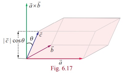
Its volume is determined by the scalar triple product (in the 3-dimensional case) of its sides $$\text{Volume} = \left( \mathbf{a} \times \mathbf{b} \right) \cdot \mathbf{c} = \begin{vmatrix} a_2 & a_3 \\ b_2 & b_3 \end{vmatrix}\,c_1 - \begin{vmatrix} a_1 & a_3 \\ b_1 & b_3 \end{vmatrix}\,c_2 + \begin{vmatrix} a_1 & a_2 \\ b_1 & b_2 \end{vmatrix}\,c_3 = \begin{vmatrix} c_1 & c_2 & c_3 \\ a_1 & a_2 & a_3 \\ b_1 & b_2 & b_3 \end{vmatrix}$$
Thus, the volume of the 3-dimensional parallelepiped is finally some $3 \times 3$ determinant of vector components of its sides. To generalise in 4 dimensions is difficult to imagine (4-dimensional volume?). A clue to it can give us the property of the determinant that if one swaps 2 rows the determinant changes sign. So, in the above determinant, we swap the first and second row and then swap the second and third row, and the determinant remains the same $$\begin{vmatrix} c_1 & c_2 & c_3 \\ a_1 & a_2 & a_3 \\ b_1 & b_2 & b_3 \end{vmatrix} = -\begin{vmatrix} a_1 & a_2 & a_3 \\ c_1 & c_2 & c_3 \\ b_1 & b_2 & b_3 \end{vmatrix} = \begin{vmatrix} a_1 & a_2 & a_3 \\ b_1 & b_2 & b_3 \\ c_1 & c_2 & c_3 \end{vmatrix}$$
This allows to generalise the volume in 4-dimensions as a $4 \times 4$ determinant $$\text{4-volume} = \begin{vmatrix} a_0 & a_1 & a_2 & a_3 \\ b_0 & b_1 & b_2 & b_3 \\ c_0 & c_1 & c_2 & c_3 \\ d_0 & d_1 & d_2 & d_3 \end{vmatrix}$$
Further generalisation using vectors and tensors is to represent the elementary volume determinant through the Levi-Civita symbol $\varepsilon^{iklm}$ which is +1 upon even permutation of indices, -1 upon odd permutation, and 0 on repeating indices.
$$dV^4 = \begin{vmatrix} d_0 x^0 & d_0 x^1 & d_0 x^2 & d_0 x^3 \\ d_1 x^0 & d_1 x^1 & d_1 x^2 & d_1 x^3 \\ d_2 x^0 & d_2 x^1 & d_2 x^2 & d_2 x^3 \\ d_3 x^0 & d_3 x^1 & d_3 x^2 & d_3 x^3 \end{vmatrix} = \varepsilon^{iklm} d_{i} x^0 d_{k} x^1 d_{l} x^2 d_{m} x^3$$Let's see how Levi-Civita symbol (tensor) changes upon change of coordinates from Gallilean $x^i$ to curvilinear $\tilde{x}^i$. First, this is done with the usual tensor transformation $$\varepsilon^{iklm} = \frac{\partial x^i}{\partial \tilde{x}^p} \frac{\partial x^k}{\partial \tilde{x}^r} \frac{\partial x^l}{\partial \tilde{x}^s} \frac{\partial x^m}{\partial \tilde{x}^t}\mathcal{E}^{prst} = \frac{\mathcal{E}^{iklm}}{J}$$ and, therefore, $\mathcal{E}^{iklm} = J \varepsilon^{iklm} = \frac{1}{\sqrt{-g}} \varepsilon^{iklm}$ (83,13 in [1]). Similarly, $\mathcal{E}_{iklm} = \sqrt{-g} \,\varepsilon_{iklm}$ (83,14 in [1]). As a second way, the volume in Galillean coordinates $\varepsilon^{iklm} d_{i} x^0 d_{k} x^1 d_{l} x^2 d_{m} x^3$ is transformed into curvilinear coordinates by transforming each coordinate as a contravariant vector as usual. $$\begin{align} d \Omega = \varepsilon^{iklm} d_i x^0 d_k x^1 d_l x^2 d_m x^3 = \varepsilon^{iklm}\frac{\partial_i x^0}{\partial_p \tilde{x}^0} d_p \tilde{x}^0 \frac{\partial_k x^1}{\partial_r \tilde{x}^1} d_r \tilde{x}^1 \frac{\partial_l x^2}{\partial_s \tilde{x}^2} d_s \tilde{x}^2 \frac{\partial_m x^3}{\partial_t \tilde{x}^3} d_t \tilde{x}^3 = \\ \varepsilon^{iklm}\frac{\partial_i x^0}{\partial_p \tilde{x}^0} \frac{\partial_k x^1}{\partial_r \tilde{x}^1} \frac{\partial_l x^2}{\partial_s \tilde{x}^2} \frac{\partial_m x^3}{\partial_t \tilde{x}^3} d_p \tilde{x}^0 d_r \tilde{x}^1 d_s \tilde{x}^2 d_t \tilde{x}^3 = \frac{\varepsilon^{iklm}}{J} d_i \tilde{x}^0 d_k \tilde{x}^1 d_l \tilde{x}^2 d_m \tilde{x}^3 = \sqrt{-g} \varepsilon^{iklm} d_i \tilde{x}^0 d_k \tilde{x}^1 d_l \tilde{x}^2 d_m \tilde{x}^3 \end{align}$$
This proves that multiplication of the volume element by $\sqrt{-g}$ makes the volume element invariant. For Galilean coordinates we have $\sqrt{-g} = 1$, so that $\sqrt{-g} d\Omega = dx\,dy\,dz\,cdt$. Further if we take an observer at rest in this Galilean system, $dx\,dy\,dz$ is his element of proper volume (3-dimensional) $dW$ and $dt$ is his proper time $d\tau/c$. Hence $\sqrt{-g} d\Omega = dW\,ds$. We see that $\sqrt{-g} d\Omega$ is the volume in natural measure of the 4-dimensional volume element. This natural or invariant volume is a physical conception – the result of physical measures made with scales unconstrained by the nature of the measured region; it may be contrasted with the geometrical volume $dV$ or $d\Omega$, which expresses the number of unit meshes that are dependent on the curvature of the selected region.
The product of the Jacobian with a scalar, vector or tensor makes the respective scalar, vector or tensor density which is usually written with gothic version of the respective letter. The power of the Jacobian is called weight $W$ of the density. If $\mathfrak{T}_{ik}$ is a rank-two tensor density of weight $W$ with covariant indices then its matrix inverse will be a rank-two tensor density of weight $−W$ with contravariant indices. As concerns determinants, from the formula: $\det{(c \mathbf{A})} = c^n \det{(\mathbf{A})}$ for a $n \times n$ matrix $\mathbf{A}$ (see Determinant), it follows that the weight of determinant is $nW$ with $n$ dimension and $W$ weight of the respective tensor.
Let $T$ be a scalar, i.e. an invariant function of position; then, since $T\sqrt{-g}\,dV$ is an invariant, $\int T\sqrt{-g}\,d\Omega$ is an invariant for any absolutely defined 4-dimensional region. Each unit mesh (whose edges $dx^1,\, dx^2,\, dx^3,\, dx^4$ are unity) contributes the amount $T\sqrt{-g}$ to this invariant. Accordingly we call $T\sqrt{-g}$ the scalar density or invariant density.
A nearly similar result is obtained for tensors. The integral $\int T^{ik}\sqrt{-g}\,d\Omega$ over an absolutely defined region is not a tensor; because, although it is the sum of a number of tensors, these tensors are not located at the same point and cannot be combined. But in the limit as the region is made infinitely small its transformation law approaches more and more nearly that of a single tensor. Thus $T^{ik}\sqrt{-g}$ is a tensor density, representing the amount per unit mesh of a tensor in the infinitesimal region round the point.
Physical quantities are of two main kinds, e.g. field of acceleration is the intensity of some condition at a point, and momentum is the quantity of something in a volume. The latter kind are naturally expressed as so much per unit mesh
. Hence intensity is naturally described by a tensor, and quantity by a tensor density. That's why we find $\sqrt{-g}$ continually appearing in our formulae; that is an indication that the physical quantities concerned are strictly tensor densities rather than tensors. In the general theory tensor densities are at least as important as tensors. We can only speak of the amount of momentum in a large volume when a definite system of coordinates has been fixed. The total momentum is the sum of the momenta in different elements of volume; and for each element there will be different coefficients of transformation, when a change of coordinates is made. The only case in which we can state the amount of something in a large region without fixing a special system of coordinates is when we are dealing with an invariant; e.g. the amount of action
in a large region is independent of the coordinates. In short, tensor analysis (except in the degenerate case of invariants) deals with things located at a point and not spread over a large region; that is why we usually have to use densities instead of quantities.
 Space-time grid (mesh) around a black hole. The unit grid reflects the curvature as the cells around the regions with strong gravitation are unequal effectively elongating space and time.
Alternatively we can express a physical quantity of the second kind as so much per unit natural volume $\sqrt{-g}\,d\Omega$
; it is then represented by a tensor. From the physical point of view it is perhaps as rational to express it in this way, as to express it by a tensor density so much per unit mesh $d\Omega$
. But analytically this is a somewhat hybrid procedure, because we seem to be employing simultaneously two systems of coordinates, the one openly for measuring the physical quantity, the other (a natural system) implicitly for measuring the volume containing it. It cannot be considered wrong in a physical sense to represent quantities of the second kind by tensors; but the analysis exposes our sub-conscious reference to $\sqrt{-g}\,d\Omega$, by the repeated appearance of $\sqrt{-g}$ in the formulae.
In any kind of space-time it is possible to choose coordinates such that $\sqrt{-g} = 1$ everywhere; for if three of the systems of partitions have been drawn arbitrarily, the fourth can be drawn so as to intercept meshes all of equal natural volume. In such coordinates tensors and tensor densities become equivalent, and the algebra may be simplified; but although this simplification does not involve any loss of generality, it is liable to obscure the deeper significance of the theory, and it is not usually desirable to adopt it. [7]
Turning our attention to metric tensor$g_{ik}$ and metric density $\mathfrak{g}^{ik}$, with $J = 1 / \sqrt{-g}$ (see the proof above), the expressions $$ J g_{ik} = \frac{g_{ik}}{\sqrt{-g}} \equiv \mathfrak{g}_{ik} \quad \text{and} \quad \frac{g^{ik}}{J} = \sqrt{-g} g^{ik} \equiv \mathfrak{g}^{ik}$$ are the covariant and contravariant metric tensor densities with weights $+1$ and $-1$, respectively.
Now this is interesting. It follows that $\mathfrak{g}_{ik} \mathfrak{g}^{il} = \frac{g_{ik}}{\sqrt{-g}} \sqrt{-g} g^{il} = g_{ik} g^{il} = \delta_{k}^{~l}$. Differentiation gives $$(\mathfrak{g}_{ik} \mathfrak{g}^{il})_{,m} = \mathfrak{g}_{ik,m} \mathfrak{g}^{il} + \mathfrak{g}_{ik} \mathfrak{g}^{il}{}_{,m} = (g_{ik} g^{il})_{,m} = g_{ik,m} g^{il} + g_{ik} g^{il}{}_{,m} = 0$$
In this respect, metric densities act very similar to metric tensors. Furthermore, it can be directly proven that $\mathfrak{g} = g$ using the formula $\left|\mathbf{AB}\right| = \left|\mathbf{A}\right| \left|\mathbf{B}\right|$. Indeed, $\mathfrak{g} = \left|\mathfrak{g}^{ik}\right| = \left|\sqrt{-g}g^{ik}\right| = \left(\sqrt{-g}\right)^4 \left|g^{ik}\right| = g^2 \cdot \frac{1}{g} = g$ .The similarity breaks, though, when we try to transform $\mathfrak{g}_{ik,l}$ and $\mathfrak{g}^{ik}{}_{,l}$ to their respective metric tensor derivatives. $$\mathfrak{g}_{ik,l} = \left(\frac{1}{\sqrt{-g}} g_{ik} \right)_{,l} = g_{ik} \left(\frac{1}{\sqrt{-g}} \right)_{,l} + \frac{1}{\sqrt{-g}} g_{ik,l} = \frac{g_{ik} g_{,l}}{2 (-g)^{3/2}} + \frac{g_{ik,l}}{\sqrt{-g}} $$ $$\mathfrak{g}^{ik}{}_{,l} = \left(\sqrt{-g} g^{ik} \right)_{,l} = g^{ik} \left(\sqrt{-g} \right)_{,l} + \sqrt{-g} g^{ik}{}_{,l} = - \frac{g^{ik} g_{,l}}{2 \sqrt{-g}} + \sqrt{-g} g^{ik}{}_{,l}$$ Reversing these equations we have for $g_{ik,l}$ and $g^{ik}{}_{,l}$ $$g_{ik,l} = \sqrt{-g} \, \mathfrak{g}_{ik,l} + \frac{g_{ik} g_{,l}}{2 g}$$ $$g^{ik}{}_{,l} = \frac{ \mathfrak{g}^{ik}{}_{,l}}{\sqrt{-g}} - \frac{g^{ik} g_{,l}}{2 g}$$ As we cannot get rid of that $g_{,l}$ the next best thing is to convert it to $\mathfrak{g}^{ik}{}_{,l}$. We already know the famous formula $g_{,l}/g = g^{ik} g_{ik,l}$ (86,4 in [1]). By the way, I have seen at least four proofs of this formula and all of them are indirect and complicated requiring differentiation of matrices which in turn necessitates decomposition into adjuncts, etc. That's why here I will give a direct and simple proof which has the additional benefit of giving us the basis for the required transformation of $g_{,l}$. I'll use the formula $\left|\mathbf{AB}\right| = \left|\mathbf{A}\right| \left|\mathbf{B}\right|$ throughout.
I'll start with $g_{ik} g^{ik} = \delta_{i}{}^{i}$ which by the above formula becomes $\left| g_{ik} \right| \left| g^{ik} \right| = \left| \delta_{i}{}^{i} \right|$, that is, $g \cdot \frac{1}{g} = 1$. In the same way $\left( g_{ik} g^{ik} \right)_{,l}= \left( \delta_{i}{}^{i} \right)_{,l}$ becomes $\left( \left| g_{ik} \right| \left| g^{ik} \right| \right)_{,l}= \left| \delta_{i}{}^{i} \right|_{,l}$ or $\left| g^{ik} \right| \, \left| g_{ik} \right|_{,l} + \left| g_{ik} \right| \, \left| g^{ik} \right|_{,l} = \frac{1}{g} \cdot g_{,l} + g \cdot \left( \frac{1}{g} \right)_{,l} = 0$. Comparing this with $g^{ik} g_{ik,l} + g_{ik} g^{ik}{}_{,l} = 0$ we see that $\frac{1}{g} \cdot g_{,l} = \frac{g_{,l}}{g} = g^{ik} g_{ik,l}$ and $g \cdot \left( \frac{1}{g} \right)_{,l} = -\frac{g_{,l}}{g} = g_{ik} g^{ik}{}_{,l}$ which is a direct proof of 86,4.
Now I'll use the proof template for $\left(\mathfrak{g}_{ik} \mathfrak{g}^{ik}\right)_{,l}$ instead of $(g_{ik} g^{ik})_{,l}$. Expanding $\left(\mathfrak{g}_{ik} \mathfrak{g}^{ik}\right)_{,l} = \mathfrak{g}_{ik,l} \mathfrak{g}^{ik} + \mathfrak{g}_{ik} \mathfrak{g}^{ik}{}_{,l} = 0$ corresponds to $\left( \left| \mathfrak{g}_{ik} \right| \left| \mathfrak{g}^{ik} \right| \right)_{,l} = \left| \mathfrak{g}^{ik} \right| \, \left| \mathfrak{g}_{ik} \right|_{,l} + \left| \mathfrak{g}_{ik} \right| \, \left| \mathfrak{g}^{ik} \right|_{,l} = \left| \delta_{i}{}^{i} \right|_{,l} = 0$. For the determinants of the metric densities I'll use the above formula for determinants $\det{(c \mathbf{A})} = c^n \det{(\mathbf{A})}$. So $$\left| \mathfrak{g}_{ik} \right| = \left| \frac{1}{\sqrt{-g}} g_{ik} \right| = \left(\frac{1}{\sqrt{-g}}\right)^4 \left| g_{ik} \right| = \frac{1}{g^2} \cdot g = \frac{1}{g}$$ $$\left| \mathfrak{g}^{ik} \right| = \left| \sqrt{-g} g^{ik} \right| = \left(\sqrt{-g}\right)^4 \left| g^{ik} \right| = g^2 \cdot \frac{1}{g} = g$$ We have the interesting result that $\left| g_{ik} \right| = \left| \mathfrak{g}^{ik} \right| = g$ and $\left| g^{ik} \right| = \left| \mathfrak{g}_{ik} \right| = \frac{1}{g}$. How will this reflect on $g_{,l}$ terms? To continue the above $\left| \mathfrak{g}^{ik} \right| \, \left| \mathfrak{g}_{ik} \right|_{,l} + \left| \mathfrak{g}_{ik} \right| \, \left| \mathfrak{g}^{ik} \right|_{,l} = g \cdot \left( \frac{1}{g} \right)_{,l} + \frac{1}{g} g_{,l}$. Comparing we get 86,4 for the metric densities but somewhat in reverse $\frac{1}{g} \cdot g_{,l} = \frac{g_{,l}}{g} = \mathfrak{g}_{ik} \mathfrak{g}^{ik}{}_{,l}$ and $g \cdot \left( \frac{1}{g} \right)_{,l} = -\frac{g_{,l}}{g} = \mathfrak{g}^{ik} \mathfrak{g}_{ik,l}$. It is easily seen why the canonical derivative for the metric $g_{ik,l}$ becomes $\mathfrak{g}^{ik}{}_{,l}$ for the densities.
In conclusion, this post gave the complete derivation of the Landau-Lifshitz pseudotensor in its various forms: in metrics, in Christoffel symbols, and in metric densities. It also explained why the metric densities formulation (Gothic metric) is preferred. The exposition was directed exclusively towards the computational technicalities and nothing was said about the physical meaning of these forms. Such physical considerations, and also a comparison of the LL pseudotensor with the closely related Synge's and Fock pseudotensors will be included in the next post.
Citation
This preprint can be cited as: Antonov, Lyudmil. Landau-Lifshitz stress-energy pseudotensor. ResearchGate DOI: 10.13140/RG.2.2.27292.36483/2
Work in progress
ReplyDelete